
The CEILING.MATH function in Google Sheets rounds a number up to the nearest integer multiple of a specified significance. Depending on the mode setting, you can round negative numbers toward or away from zero.
CEILING.MATH and CEILING.PRECISE are newer, improved versions of the CEILING function.
Syntax
=CEILING.MATH(number, [significance], [mode])
number – The number for the function to round.
significance – Optional. The multiple to round up to. The default value is 1.
mode – Optional. The rounding direction for negative numbers. This has no impact on positive numbers.
0– Default value. Round toward zero1– Round away from zero
Similar Functions
Several functions deal with rounding. Choose the most appropriate for your use.
- CEILING.MATH – Rounds a number up to the nearest integer multiple of specified significance with custom negative number treatment
- CEILING.PRECISE – Rounds a number up to the nearest integer multiple of specified significance
- INT – Rounds a number down to the nearest integer
- FLOOR.MATH – Rounds a number down to the nearest integer multiple of specified significance with custom negative number treatment
- FLOOR.PRECISE – Rounds a number down to the nearest integer multiple of specified significance
- MROUND – Rounds a number to the nearest multiple of another number
- ROUND – Rounds a number to a specified number of decimal places using standard rounding
- ROUNDDOWN – Round a number down to a specified number of places
- ROUNDUP – Round a number up to a specified number of places
- TRUNC – Truncates a number to a certain number of significant digits by omitting less significant digits
Insert Math Symbols (Add-On)

Possible Errors
#VALUE! – An argument is non-numeric.
Examples
You can use CEILING.MATH in many different ways. Let’s take a look at a few, starting with rounding currency.
Example 1 – Round Up to the Next Nickel
Sometimes, presenting a price rounded up to the next nickel looks better. Let’s look at how to do that.

The formula used in cell C2: =CEILING.MATH(A2,B2)
We use the CEILING.MATH function to round the Original Price to a significance of $0.05. Google Sheets does not round the value in row 3 because $1.25 is already a multiple of $0.05. Since the function rounds up, it rounds $1.23 up to $1.25 in row 2 and rounds $1.27 up to $1.30 in row 4.
Example 2 – Round Up to the Nearest Half-Hour
Next, let’s round some time values. It is common to refer to a time as a rounded value. In this example, we’ll round values up to the next half-hour.
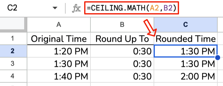
The formula used in cell C2: =CEILING.MATH(A2,B2)
⚠️ You can enter a half hour as “0:30” or “0:30:00“.
Rows 2 and 4 both get rounded up to the next half hour. Since the 1:30 PM in row 3 is already a multiple of 30 minutes, the CEILING.MATH function does not change it.
Example 3 – Round With Different Significances
Up to this point, we have been changing the number. Now, let’s look at changing the significance. We’ll use positive and negative significances to see the difference.

This example shows us why the function has a mode argument. You can see that positives move away from zero while the negatives move toward zero. If you want negative values to move away from zero, you must change the value of the mode argument. Let’s look at that in the following example.
Example 4 – Rounding Negative Numbers with Different Modes
In previous examples, we did not specify a value for the mode argument. Now, we will use it to instruct the function in which direction to round negative values.

In rows 2 through 4, the mode of 0 makes the function round negative values toward zero. Specifying a mode of 1 (or anything other than zero) moves the values away from zero.
Live Example in Sheets
Make a copy of this spreadsheet to get the examples in your Google Drive.