
The COUNTUNIQUEIFS function counts the unique values that meet multiple criteria in Google Sheets. This function accepts a variable number of arguments, each consisting of a range of cells and corresponding criteria.
It is similar to the COUNTIFS function, which also accepts multiple criteria. However, COUNTUNIQUEIFS counts unique values, whereas COUNTIFS counts all values that meet the specified criteria.

Contents
Syntax
=COUNTUNIQUEIFS(range, criteria_range1, criterion1, [criteria_range2, …], [criterion2, …])
range – The cells with the unique values
criteria_range – The cells to evaluate against the criterion
criterion – The condition to apply to the criteria_range
Insert Math Symbols (Add-On)

Similar Functions
COUNT – Count the numeric values in a data set
COUNTA – Count the non-blank values in a data set
COUNTIF – Count the cells that match a criterion
COUNTIFS – Count the cells that match multiple criteria
COUNTUNIQUE – Count the unique values
COUNTUNIQUEIFS – Count the unique values that meet multiple criteria
COUNTBLANK – Count the blank cells
Examples
Example 1 – Conditionally Counting Unique Values With One Criterion
Firstly, let’s start with an example of counting unique values based on one condition.

Formula used: =COUNTUNIQUEIFS(A2:A13,B2:B13,"East")
The first argument, A2:A13, specifies the range of cells to count. The second and third arguments, B2:B13 and "East" are the criteria_range containing the data to check against the criterion.
In other words, the COUNTUNIQUEIFS function counts the number of unique items in the East warehouse.
Let’s look at another example using one criterion from a different angle.
Example 2 – Conditionally Counting Unique Values With One Criterion
Let’s keep the same source data but look for the number of warehouses with wrenches. This example will help us to understand how to build different formulas to analyze the same data.

Formula used: =COUNTUNIQUEIFS(B2:B13,A2:A13,"Wrench")
To find how many warehouses are stocking Wrenches, we will switch the values of the range and criteria_range from the first example. We want to count unique values in the range of B2:B13 if they match the criterion of "Wrench" in the criterian_range of A2:A13.
In other words, how many warehouses have wrenches in stock?
Last but not least, let’s look at a more complex example.
Example 3 – Conditionally Counting Unique Values With Two Criteria
Lastly, we will look for unique values based on the satisfaction of two conditions.
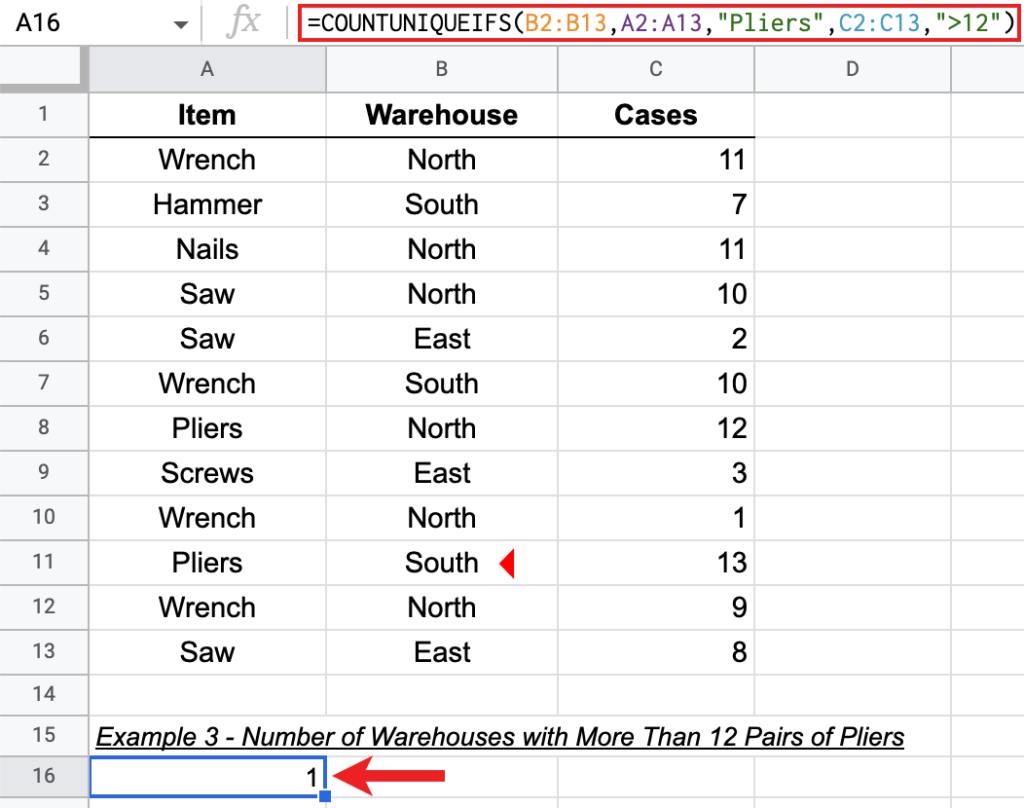
Formula used: =COUNTUNIQUEIFS(B2:B13,A2:A13,"Pliers",C2:C13,">12")
As we increase the criteria, we start to see the power of the COUNTUNIQUEIFS function. In this example, we are looking for locations that have more than 12 cases of pliers. We count the warehouses by specifying B2:B13 as the range, then using A2:A13 and C2:C13 as the criteria_ranges.
As an interesting twist, since there was only one situation with more than 12 cases of Pliers, we would get the same result using the COUNTIFS function.
Live Example in Google Sheets
Make a copy of this spreadsheet to see the examples in the live web app.
Video Tutorial

Related Tutorials
-
Conditionally Count Unique Values in Google Sheets
Three techniques to count unique values based on specified criteria.