30/360, Actual/365, and Actual/360 Day Counts

Lenders can choose different methods to count the days when calculating loan interest. What should be a straightforward exercise becomes more involved with these differences. Let’s take a deeper look.

We will examine the 30/360, actual/365, and actual/360 day counting conventions. As we go through the examples, you can follow along with the spreadsheet we used. You will see that each method results in a different amount of interest.

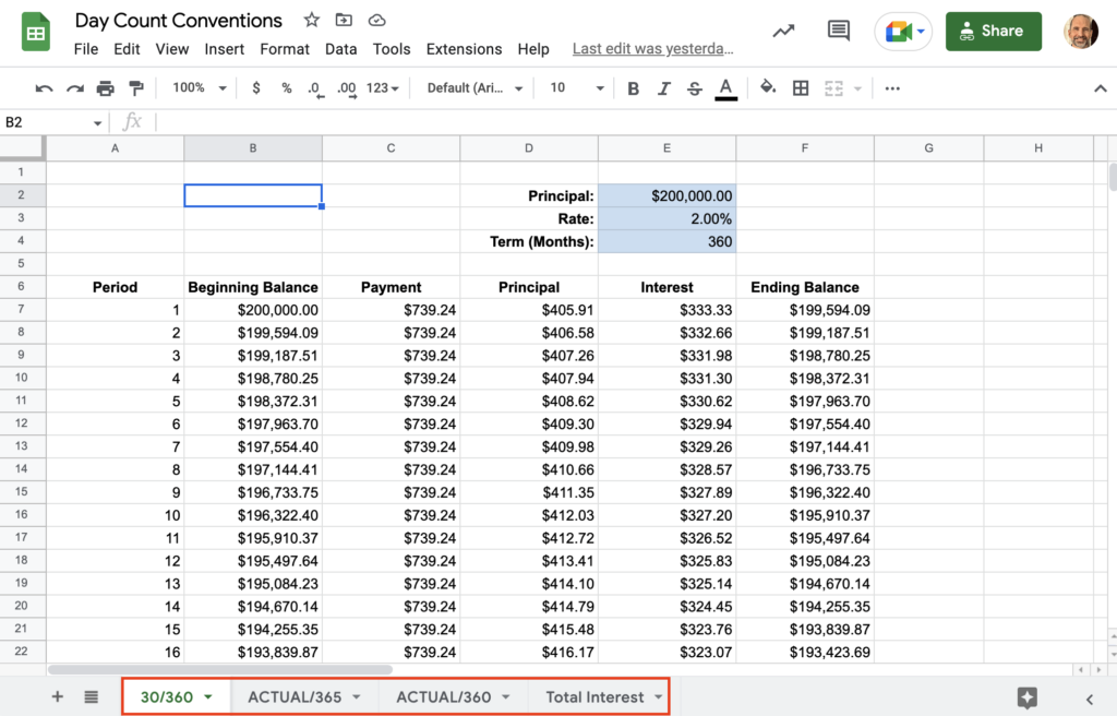
The example Google Sheet has a tab for each method and one for comparing the interest.

Each day count method has a 360-month (30-year) amortization schedule. Each note has a principal of $200,000 and a rate of 2.00%. Keeping these values constant throughout the three schedules enables a fair comparison. The difference between the schedules is the interest calculation. Now let’s look at the 30/360 calculation used in the first worksheet.

Video Tutorial

30/360 Day Count Convention

The 30/360 day count convention is the simplest method of the three.

The formula used in cell E7 for interest charged is:

=B7*(E$3*30/360)

The first input to the formula is the period’s beginning balance in cell B7. Column B‘s values are reduced each period by the principal repayments in column D. Since period 1 is the first period, this formula uses $200,000 for this value.

E$3 references the rate for every row. The $ fixes the row reference, so it does not shift down when you copy the formula.

The last part of the interest formula is 30/360, which applies the interest evenly regardless of the number of actual days in the month. Notice that 30/360 is the same as dividing the interest by 12.

Actual/365 Day Count Convention

The next convention for counting days is actual/365.

The formula used for interest is:

=(DAY(B8)/365)*F$3*C8

The calculation uses the DAY function to return the number of days each month. For example, January always returns 31 days while the result for February is either 28 or 29, depending on leap year.

Next, we divide the number of days in the month by 365. We used 365 regardless of leap year.

After using (DAY(B8)/365) to arrive at the portion of a year, we then multiply by the rate in F3 (while fixing the row with a $), then multiply by the period’s beginning balance in C8.

Actual/360 Day Count Convention

Lastly, we will look at the actual/360 day count convention. This method is one to watch out for as it effectively charges interest for five extra days each year.

The formula used for the actual/360 interest is:

=((DAY(B8)/360)*F$3*C8)

Similar to the previous example, the calculation uses the DAY function to return the number of days each month.

Next, we divide the number of days in the month by 360 instead of 365. Using a smaller denominator will make the result of the formula larger, thus charging more interest.

After using (DAY(B8)/365) to arrive at the portion of a year, we then multiply by the rate in F3 (while fixing the row with a $), then multiply by the period’s beginning balance in C8.

Difference in Interest Charges

The last sheet in the example file shows the difference in the amount of interest charged between the three methods. As you can see, 30/360 and actual/365 are similar, and the actual/360 method charges more.

Method	Interest
30/360	$66,126
Actual/365	$66,163
Actual/360	$67,165

The difference in interest charges over thirty years between 30/360 and actual/360 is $1,039. Since we’re using Google Sheets, let’s make a chart showing the difference. With some adjustment of the horizontal axis’ min and max, the chart can accentuate (or exaggerate) the difference.

Conclusion

It helps to be aware of the impact these different day count conventions can have on your loan. Think twice if your bank wants to calculate interest using the actual/360 method.

Related Tutorials