
The ISDATE function in Google Sheets is a logical function that returns TRUE if the given value is a valid date and FALSE otherwise. You can use it to validate data, perform calculations on dates, and create conditional formatting rules.
Syntax
The syntax for the ISDATE function is:
=ISDATE(value)
value: The cell reference or value that you want to check.
Related Functions
ISBLANK– Determines if a cell is emptyISDATE– Determines if a value is a valid dateISERROR– Determines if a value is an errorISERR– Determines if a value is an error other than #N/AISNA– Determines if a value is an #N/A error
ISFORMULA– Determines if a value is a formula (whichTYPEcannot do)ISLOGICAL– Determines if a value is booleanISNONTEXT– Determines if a value is not textISNUMBER– Determines if a value is a numberISREF– Determines if the value is a valid referenceISTEXT– Determines if a value is textISURL– Determines if a value is a valid website address
Examples
Here are some examples of how to use the ISDATE function:
Example 1 – Check if a Specific Date Is Valid
Let’s start simply and see if “10-11-2023” is a date. Notice that you must surround any dates in quotes if you input them directly into the function. Read more about how to use dates in formulas to learn more.
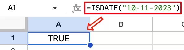
Formula used: =ISDATE("10-11-2023")
The ISDATE function returns TRUE because "10-11-2023" is a valid date format.
Struggling with dates from an import?
Manually finding bad dates with ISDATE is a common step after importing data from other calendars (like iCal, .ics, or CSVs). These imports often format dates as text, leaving you to clean up the mess.
Our Calendar Importer add-on solves this. It intelligently parses and imports your calendar events directly into Google Sheets with the correct date formats automatically.
Example 2 – Check if a Cell Contains a Valid Date
Next, let’s use a cell reference as input.
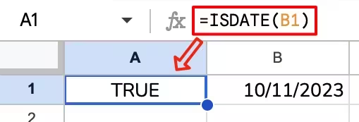
Formula used: =ISDATE(B1)
In this formula, Google Sheets looks at the value in cell B1, determines it is a date, and returns TRUE.
Example 3 – Validate a Data Range
You can use the ISDATE function to ensure that all values in a range are valid dates. Let’s do that for columns B and C below.
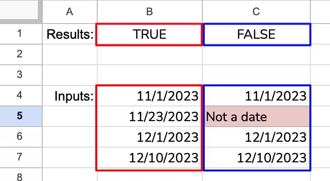
Formula in cell B1: =ISDATE(B4:B7)
Formula in cell C1: =ISDATE(C4:C7)
If any values in the two ranges are not valid dates, the formula will return FALSE. All the values in B4:B7 are valid dates, so the formula in cell B1 returns TRUE. However, the value in C5 is not a date, so the formula in cell C1 returns FALSE.
Example 4 – Create Conditional Formatting Rules
You can use the ISDATE function to create conditional formatting rules. For example, you could highlight all of the cells in a range that contain invalid dates using the following conditional formatting rule:
Format cells if...
Custom formula is:
=NOT(ISDATE(A1))
This is what the formula looks like in Google Sheets when entered as a conditional formatting rule.
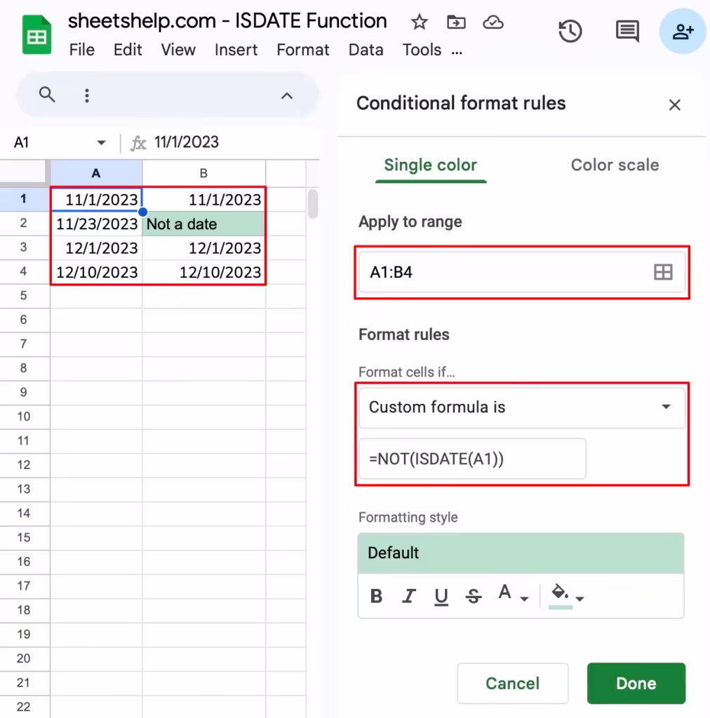
The completed conditional formatting rule changes the background fill of cell B2 to green because it is not a valid date.
Frequently Asked Questions
Q: Why is ISDATE returning FALSE for a date? A: This usually happens when the “date” is actually a text string that just looks like a date (e.g., from a data import). You can also check your spreadsheet’s “Locale” setting (under File > Settings), as it might be expecting a different format (like MM/DD/YYYY vs. DD/MM/YYYY).
Q: How can I check if a cell is a date OR is blank? A: You can combine ISDATE with the OR and ISBLANK functions, like this: =OR(ISDATE(A1), ISBLANK(A1))
Live Examples in Google Sheets
Get a copy of the spreadsheet with these examples to use yourself.
Conclusion
The ISDATE function is a powerful tool for validating data. By understanding how to use it, you can improve the accuracy of your spreadsheets. And if your date validation problems come from importing external calendars, save yourself the hassle of manual cleanup and let Calendar Importer handle it for you automatically.