
NETWORKDAYS.INTL calculates the number of working days between two dates. The function excludes weekends (which may or may not be Saturday and Sunday) and can optionally exclude holidays.

If your weekends are Saturday and Sunday, consider using the simpler NETWORKDAYS function.
⚠️ The start_date and end_date are included in the count of days.
Contents
Syntax
=NETWORKDAYS.INTL(start_date,end_date,[weekend day(s)],[holiday(s)])
start_date The date at which to start the counting
end_date The date at which to end the counting
[weekend day(s)] An optional description of which days are weekends.
- Number method
- 1 – Saturday and Sunday [don’t need to specify]
- 2 – Sunday and Monday
- 3 – Monday and Tuesday
- 4 – Tuesday and Wednesday
- 5 – Wednesday and Thursday
- 6 – Thursday and Friday
- 7 – Friday and Saturday
- 11 – Sunday only
- 12 – Monday only
- 13 – Tuesday only
- 14 – Wednesday only
- 15 – Thursday only
- 16 – Friday only
- 17 – Saturday only
- String method – Each digit represents a day. The first digit is Monday. Some examples are as follows:
- 0000011 – Saturday and Sunday
- 0100000 – Only Tuesday
[holiday(s)] An optional list of holidays to exclude from the count of days.
Related Functions
DAYS – Calculate the number of days between two dates.
DATEDIF – Calculate the time between two dates in years, months, or days.
MINUS – Subtract one value from another. The MINUS function can subtract dates.
NETWORKDAYS – Calculate the number of working days without the weekend modifications of NETWORKDAYS.INTL
Errors
#VALUE! – An input(s) isn’t a valid date such as “The other day” or “Yester-yester-day”.
Examples
Example 1 – One Day Weekends (1st Method)
In this first example, we specify that only Sundays are weekends.

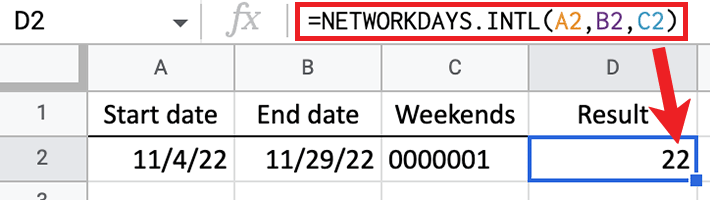
Formula used: =NETWORKDAYS.INTL(A2,B2,C2)
We tell Google Sheets to only use Sundays as weekends by using an 11 for the weekend code. In this example’s formula, we do this by referencing cell C2 which contains the number 11.

This calendar shows us which days are counted. Each full week has six workdays and after accounting for the two partial weeks, we come to 22 workdays.
? See this video to learn about the pop-up calendar in Google Sheets.
Example 2 – One Day Weekends (2nd Method)
There is a more intuitive technique for specifying weekends.
Formula used: =NETWORKDAYS.INTL(A2,B2,C2)
With this technique, you can use a text string of seven digits like in cell C2. In this string, a 0 indicates a workday, and a 1 indicates weekends. Each digit’s location inside the seven-digit string indicates the day of the week, with the first digit being Monday. Notice the apostrophe before the seven numbers. This tells Sheets to treat the value as text instead of a number.

Since both examples 1 and 2 use Sundays as weekends, they each result in 22 workdays.
Example 3 – Custom Weekends and a Holiday
Similar to the NETWORKDAYS function, NETWORKDAYS.INTL lets you specify holidays. The holidays argument is optional, so leave it off if you don’t have any in your calculation.

Formula used: =NETWORKDAYS.INTL(A2,B2,C2,D2)
The holiday is placed in cell D2. As seen in the calendar, the Sunday weekends and the holiday of November 24th are excluded.
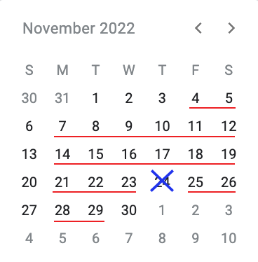
With the holiday subtracted, there are 21 workdays between November 4 and November 29, 2022.
Live Examples in Sheets
Go to this spreadsheet for examples of the NETWORKDAYS.INTL function shown above that you can study and use anywhere you would like.
Notes
Consider using the IMPORTXML function to obtain a list of your local holidays online.
Use the Calendar Importer tool to import start and end days and times from events in Google Calendar.
Video Tutorial
