
RANK.AVG is a statistical function in Google Sheets that assigns a position to a value within a set of values. It is handy for ranking data in ascending or descending order and identifying a dataset’s top or bottom values.
ℹ️ This function and RANK.EQ replace the older RANK function with more specific capabilities. RANK.EQ shows ties as the same rank while RANK.AVG provides the average rank. You will see average ranks in examples 2 and 3 below.
Contents
Syntax
The syntax for the RANK.AVG function is as follows:
=RANK.AVG(value, data, [is_ascending)
value– The value whose rank you want to determine.data– The range of cells containing the dataset to rank.is_acending– An optional parameter that specifies the ranking direction0– Default value. The largest value is ranked 1.1– The smallest value is ranked 1.
Similar Functions
RANK – Shows the rank of a value in a set of values. This function is old. Use RANK.AVG or RANK.EQ instead.
RANK.EQ – Shows the rank of a value in a set of values. RANK.EQ is a replacement function for RANK.
SORTN – Creates a sorted list of the top n values from a data set
Common Errors
#VALUE! – An input is something other than a number. Check the input values to ensure they are all numbers.
#N/A! – No valid input data. Possible causes include the value not in the data or a blank value.
Examples
Here are three examples of how to use the RANK.AVG function in Google Sheets:
Example 1 – Simple Ranking
Suppose you have a dataset of sales figures for different products and want to rank them based on their sales. You can use the following formula to rank the products in descending order:
Formula in cell C2 =RANK.AVG(B2, B$2:$B4)
Where:
B2is the cell reference for the sales figure of the first product.B$2:B$4is the cell range containing the sales figures for all products.
You don’t need to specify the is_ascending argument to rank the largest amount first. Therefore, we only need the value and data inputs for this example. Note the $s used in the range. Using $s fixes the reference so the row numbers do not change when you copy the formula into C3 and C4.
Example 2 – How to Rank Equal Amounts (Ties)
Next, suppose you have student grades and want to identify the top students in the class. You can use the following formula to identify the top students.
Formula in cell C2 =RANK.AVG(B2,B$2:B$5)
Where:
B2is the cell reference containing the grade of the first studentB2:B5is the cell range containing the student grades.
However, notice that there are two students with an 87%. This function gives both students a rank of 2.5, the average of 2 and 3, and assigns a 4 to the 75% since it is the fourth highest score.
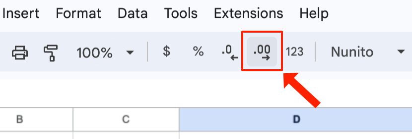
Be sure to increase the decimal places of your numbers in the toolbar, as shown above, if you are not seeing the decimal values.
Example 3 – Rank All Amounts with One Formula
Previously, we used one formula for each row in examples 1 and 2 to keep things simple. However, you can use the ARRAYFORMULA to repeat the ranking formula for multiple rows. ARRAYFORMULA lets you use a range for the value argument instead of just a cell.
Let’s redo example 2 with one formula.
Formula used in cell C2 =ARRAYFORMULA(RANK.AVG(B2:B5,B2:B5))
Live Examples in Google Sheets
Make a copy of this Google Sheet to see the formulas in action.
Tips for using the RANK.AVG function
- If the
datarange contains duplicate values, this function will assign the same rank to all identical values. - If the
datarange includes empty cells, the RANK.AVG function will ignore the empty cells.
Video Tutorial

Conclusion
The RANK.AVG function is a powerful tool for analyzing data in various ways. By understanding how to use the RANK.AVG function, you can perform more sophisticated calculations and identify trends and patterns in your data that you may not have been able to see before.