Sum Values Based on Another Cell’s Values in Google Sheets

Google Sheets offers a variety of methods to sum amounts based on values in other cells. These techniques can be helpful for many different tasks, such as calculating sales by region, product, or customer; tracking expenses by category; or summarizing financial data. The solutions in this article will start simple and get more complex as we go.

📼 This tutorial is easier to understand in video form.

We will use this table of data for all the examples. This table, along with the solutions, are in this linked Sheet if you want to follow along.

First, we’ll start with a technique that uses two functions that you may already know.

Example 1 – Sum Values With Traditional Functions

Our goal is to find how many cases there are of each Item. We will end up with a list of the Items in one column and total Cases in the next column. We’ll use two functions to get this done. First, we’ll use the UNIQUE function which returns a list of unique values from a range.

UNIQUE Syntax: =UNIQUE(range)

We’ll give the UNIQUE function the range where the Items reside, which is A2:A11. This function will return a list of the unique Items from this range. Notice we did not include row 1.

⚠️ You need to type the headers when using this function.

Now we have a list of the four unique Items we want to sum. Now, we will use the SUMIF function.

The SUMIF function is one of the most common ways to sum amounts based on values in other cells. It takes three arguments: the range of cells containing the criterion, the criterion used to filter the cells, and the range of cells to be summed (sum_range).

SUMIF Syntax: =SUMIF(range, criterion, [sum_range])

=SUMIF($A$2:$A$11,E2,$B$2:$B$11)

The formula in cell F2 calculates the total of all values in column B, but only for rows where column A contains “Wrench“. By using fixed cell references for the range and sum_range, you can duplicate this formula in cells F3, F4, and F5. When you do this, the ranges will remain constant, but the Item being searched for will change to match the corresponding cell in column E.

That is the simplest way to add values based on other cells. Let’s look at using a pivot table next, which gives us more flexibility than using UNIQUE and SUMIF.

Example 2 – Sum Values Using Pivot Tables

Pivot tables are a powerful tool for summarizing and analyzing data. You can use them to sum amounts based on values in other cells, as well as to calculate other statistical measures, such as averages, medians, and counts.

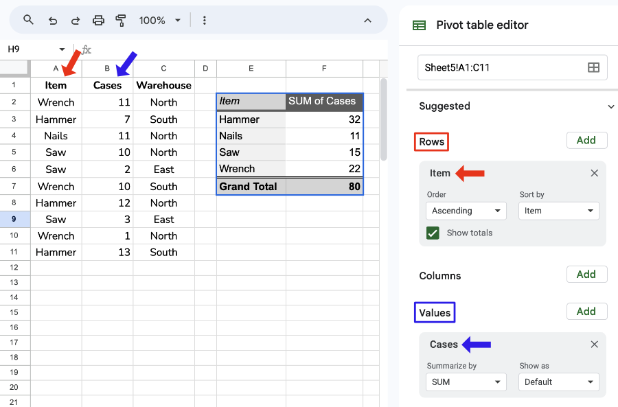
For this example, we will use a pivot table to create the same output as in step one, but without any formulas.

To create a pivot table, select the range of data you want to analyze, and then click on the Insert menu and select Pivot table. Use the OmniPivot add-on to use more than one range. The Insert and Pivot table menu combination opens the pivot table editor.

In the pivot table editor, drag the fields you want to use to summarize the data to the Rows, and Values areas. For this example, to sum the Items in column B for each unique Item listed in column A, drag the Item field to the Rows area and the Cases field to the Values area in the pivot table editor.

Once you have created the pivot table, you can filter the data and calculate subtotals and grand totals as needed. Let’s look at another flexible solution next.

Example 3 – Sum Values Using the QUERY function

The QUERY function is a powerful tool for filtering and sorting data. You can also use it to sum amounts based on values in other cells.

For example, to sum the Cases in column B for the Items listed in column A, you would use the following formula:

=QUERY(A1:C11,"select A, sum(B) group by A",1)

This formula will return the sum of all of the Cases in column B where the corresponding Item in column A is equal to that Item. Unlike example 1, one formula creates these results. Also, the QUERY lets you use SQL-like commands, opening up new possibilities not available in traditional spreadsheet functions.

Example 4 – Sum with More than One Condition

You may wonder why you should use a less familiar solution like the QUERY function in example 3. That question is easy to answer by showing what happens when you add another condition. Let’s look at summing the values by Item then by Warehouse. This extra level of summing would need many more formulas if you were using SUMIF and UNIQUE, like in example 1. But, using the QUERY function, you still need only one formula.

=QUERY(A1:C11,"select A, C, sum(B) group by A, C",1)

We added another layer simply by adding a few letters to the QUERY formula.

Video Tutorial

Conclusion

Google Sheets offers a variety of ways to sum amounts based on values in other cells. The best method to use will depend on the specific needs of your task.

To create a list of unique values from a range of cells, you can use the UNIQUE function. You can then use this list with SUMIF to sum amounts based on the unique values in another column. Pivot tables are a powerful tool for summarizing and analyzing data, and you can also use them to sum amounts based on values in other cells. The QUERY function is a powerful tool for filtering and sorting data, and you can also use it to add amounts based on values in other cells.

Related Articles