The TEXT function in Google Sheets is a powerful and flexible function that allows you to format numerical data in various ways. It converts a number to a specific format, such as dates and times, an integer with a thousands separator, or even a number rounded to a significant digit.
⚠️ The TEXT function creates a text string, not a number. Use number formatting to change the format of a number without changing it to a text string.
The TEXT function overrides any formatting applied to the cell.
Contents
Syntax
=TEXT(value, format)
value– A numeric value
format– The number format for the output- See customformats.com for a comprehensive listing of number formats.
Related Functions
CONCATENATE – Join strings together
DATEVALUE – Accepts a date value in any valid format and returns it as a serial number
TIMEVALUE – Converts a time to a numeric value. Similar to DATEVALUE.
VALUE – Converts a number string into a number (the opposite of this function)
Examples
Here are some examples of how you can use the TEXT function in Google Sheets:
Example 1 – Two Decimal Places
First, we’ll use the TEXT function to convert a number to a number string with a specific format.

=TEXT(value,"0.00")
These formulas convert the numbers to text with two decimal places.
Example 2 – U.S. Date Format
Next, we’ll format dates into a standard United States date syntax.

=TEXT(value,"MM/DD/YYYY")
This formula will format the dates as “Month/Day/Year” with the month and day always being two digits and the year being four digits.
Example 3 – Currency
Now let’s convert numbers to a currency format.

=TEXT(value,"$#,##0.00")
This formula formats the value as currency, with a dollar sign and two decimal places.
Example 4 – Duration
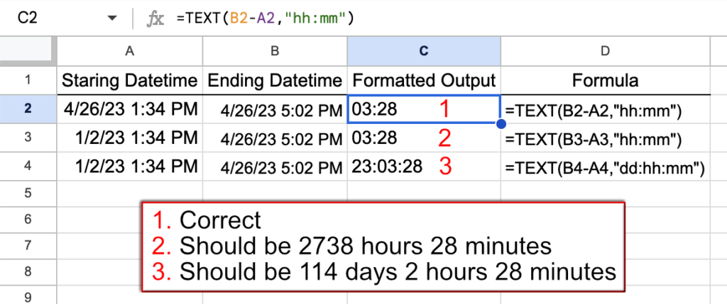
Lastly, let’s look at formatting durations. We’ll look at short durations of under a day and longer durations. This example shows a limitation of datetime formatting and an alternative method to get the output you need.

In row 2, the duration displays correctly. There are three hours and twenty-eight minutes between the times in cells A2 and B2. However, the result of 03:28 for row 3 is incorrect. It appears to be missing 114 days. But, adding days into the formatting as we have in row 4 doesn’t fix the problem.
Let’s use the TIMEDIF add-on to find the correct durations. TIMEDIF is an add-on developed by SheetsHelp with a 7-day free trial. Let us know how it works for you.
Notice that TIMEDIF subtracted an hour from the two multi-day durations to account for daylight savings time.
Example 5 – Concatenation
When you join two numbers, the formatting can be lost. Let’s use TEXT to keep the formatting intact.

Formula used: =TEXT(A2,"H:MM AM/PM")&" and "&TEXT(A3,"H:MM AM/PM")
By formatting each value with the TEXT function before they are concatenated, you can control the formatting of the output. In this case, we used a 12-hour AM/PM time.
See these examples by copying this Google Sheets file.
