
The TRUNC function in Google Sheets removes unwanted digits from a number.
This function can simplify large numbers or convert decimal values to integers. You can also use it to filter data in a spreadsheet.
⚠️ The TRUNC function is similar to the INT function, but TRUNC accepts a place argument and treats negative numbers differently (see example 2).
Contents
Syntax
The syntax for the TRUNC function is:
=TRUNC(value, [places])
value – The number to truncate.
places – An optional argument specifying the number of digits.
Similar Functions
Several functions deal with rounding. Choose the most appropriate for your use.
- CEILING.MATH – Rounds a number up to the nearest integer multiple of specified significance with custom negative number treatment
- CEILING.PRECISE – Rounds a number up to the nearest integer multiple of specified significance
- INT – Rounds a number down to the nearest integer
- FLOOR.MATH – Rounds a number down to the nearest integer multiple of specified significance with custom negative number treatment
- FLOOR.PRECISE – Rounds a number down to the nearest integer multiple of specified significance
- MROUND – Rounds a number to the nearest multiple of another number
- ROUND – Rounds a number to a specified number of decimal places using standard rounding
- ROUNDDOWN – Round a number down to a specified number of places
- ROUNDUP – Round a number up to a specified number of places
- TRUNC – Truncates a number to a certain number of significant digits by omitting less significant digits
Possible Errors
#VALUE! – An argument is non-numeric.
Insert Math Symbols (Add-On)

TRUNC Function Examples
Here are some examples of how you can use the TRUNC function in Google Sheets:
Example 1 – Lower a Decimal to a Whole Number
To change the number 12.345 to 12, you would use the following formula:
=TRUNC(12.345)
As you can see from the result of 12, TRUNC does not follow standard rounding rules. It simply removes numbers to arrive at the number of places specified. In this case, places defaulted to 0. We’ve seen this work with a positive number. Next, let’s look at a negative number.
Example 2 – Negative Number
Next, let’s look at using TRUNC on a negative number. We’ll switch the sign to -12.345 and keep the places argument at the default of 0.
=TRUNC(-12.345)
The result is -12. It is essential to realize this is a different result than rounding a number with the INT function, which would have returned -13.
Example 3 – Filtering by Numbers
You can use this function to FILTER data in a spreadsheet. For example, the following formula would return all of the rows in a spreadsheet where the value in the Price column is an integer:
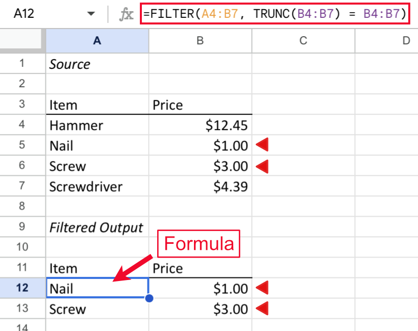
Formula used: =FILTER(A4:B7, TRUNC(B4:B7) = B4:B7)
The filter returns rows where the truncated number is the same as the original. The values only meet this condition when they have no decimal values.
Example 4 – Similarity to the ROUNDDOWN Function
Google Sheets offers many functions to handle rounding. ROUNDDOWN functions the same as the TRUNC function. Let’s look at a few values and places to show how the output compares.

As you can see, the two functions output the same results.
Live Examples in Google Sheets
Use a copy of this live Google Sheet for a quick start with the examples from above.
Conclusion
The TRUNC function in Google Sheets helps remove decimal places from numbers. This function can make numbers easier to read and understand or work with in calculations.