
Spreadsheets allow you to make sense of complex sets of numbers quickly. In this post, we’ll give you the skills to find the smallest value in your data while filtering the values before you evaluate them. We’ll use a real-world example of examining inventory. We have a list of Prices in column A and a list of their Status in column B.
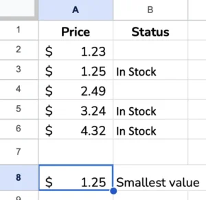
We want to find the lowest price for our In Stock items. Therefore, we need a way to filter the values so we can only consider those In stock before we look at the prices.
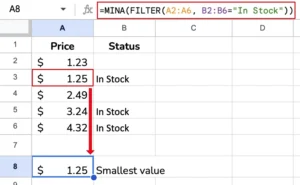
=MINA(FILTER(A2:A6, B2:B6="In Stock"))
This formula combines the MINA function with the FILTER function in Google Sheets.
Here’s how it works step-by-step:
- The
FILTERfunction evaluates the rangeA2:B6and includes the rows where the text inB2:B6is “In Stock.” - This filtered range of values from column
Ais then passed as the argument to theMINAfunction. MINAwill then find the minimum value across that filtered range from columnA.
So, in essence, this formula is:
- Identifying the products that are “
In Stock” by looking at the values in columnB - Taking only the prices for those in-stock products from column
A - And then finding the lowest price from that filtered set of in-stock prices
This can be useful when determining the minimum value, but only for a specific subset of the data. In this case, it’s finding the lowest price among the In-stock items.
The FILTER function allows you to apply conditional logic to select the relevant data before passing it to MINA (or other functions). This makes the MINA result more targeted and meaningful.
Make a copy of the spreadsheet used in this example to adapt the formulas to your spreadsheet.
Related Tutorials
-
SUMIFS Function – Google Sheets
The SUMIFS function adds numbers if multiple conditions are true. All conditions must be met for the function to sum a value, and all ranges must be the same size. You can use SUMIF to check for one condition. Feel free to copy the template with these examples to follow along. Contents1 Purpose2 Syntax3 Related Functions4 Video…
-
SUMIF Function – Google Sheets
The SUMIF function is used in Google Sheets to add numbers if data meets a specific condition. Use SUMIFS to check for multiple conditions. Feel free to copy the template with these examples to follow along. Contents1 Purpose2 Syntax3 Related Functions4 Video Tutorial5 Common Error6 Examples6.1 Example 1 – Sum Values Greater Than or Equal to an…
-
Sharing And Protecting Your Google Sheet
Sharing and protecting your file starts with clicking the green Share button or using the File option in the menu bar, then choosing Share. From the sharing menu, you have two main options. Firstly, you can invite other users or, secondly, create a link to share your spreadsheet. Contents1 Video Tutorial2 Share with People and…