Google Sheets is a powerful spreadsheet application that you can use to track a variety of data, including work hours between two dates. To calculate the business hours between two days in Google Sheets, you can use the following steps.
This is perfect for freelancers tracking billable meeting time, teams analyzing time spent in project meetings, or anyone who wants to see “how many hours did I actually work last month?” without manual data entry.
Contents
- 1 Steps to Calculate Hours
- 2 Automate with Calendar Data
- 3 FAQ
- 3.1 Does NETWORKDAYS count weekends?
- 3.2 What if I work different hours on different days?
- 3.3 Why is my result showing a #VALUE! error?
- 3.4 Can I exclude multiple holidays?
- 3.5 What if my work week is 4 days instead of 5?
- 3.6 How do I calculate work hours for multiple employees or projects?
- 3.7 The formula is counting one extra or one fewer day than expected. Why?
- 4 Live Example in Sheets
- 5 Similar Posts
Steps to Calculate Hours
Define Your Inputs
For this example, we will use the following inputs.
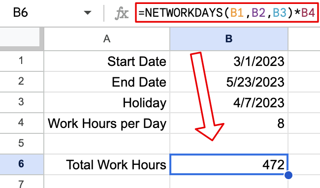
start_date: March 1, 2023end_date: May 23, 2023holidays: April 7, 2023work_hours_per_day: 8
Make of copy of the example spreadsheet and change any of the inputs to fit your situation.
Add The NETWORKDAYS Function
First, find the number of workdays less any holidays. The NETWORKDAYS function is the perfect fit for this.
Syntax: =NETWORKDAYS(start_date, end_date, holidays)
Using a start_date of 3/1/2023 and an end_date of 5/23/2023, the formula counts 60 workdays. Then, the formula subtracts 4/7/2023 for Good Friday, leaving 59 workdays. Now that we have the number of work days, let’s convert the work days to work hours.
Multiply by Work Hours Per Day
Now that you have the number of workdays, multiply that number by the number of work hours in each work day.
Syntax: =NETWORKDAYS(start_date, end_date, holidays) * work_hours_per_day

This formula multiplies the 59 days we found in the previous step by 8 work hours per day. This multiplication results in 472 work hours between 3/1/2023 and 5/23/2023.
⚠️ Consider using NETWORKDAYS.INTL if you need to specify custom weekends.
 Automate with Calendar Data
Manually entering start and end dates works great for planned calculations, but what if you’re tracking hours that already exist in Google Calendar?
You can import calendar events directly into Google Sheets and then use the formula above to calculate total work hours automatically. This is perfect for freelancers tracking billable meeting time or teams analyzing time spent in project meetings.
The Calendar Importer for Google Sheets add-on pulls your events into a spreadsheet where each row contains start time and end time. From there, apply the NETWORKDAYS formula to calculate work hours across any date range.
FAQ
Does NETWORKDAYS count weekends?
No, NETWORKDAYS automatically excludes Saturdays and Sundays from the calculation. It only counts Monday through Friday as workdays. If you need to specify a custom work week (like Sunday-Thursday or a 4-day work week), use the NETWORKDAYS.INTL function instead.
What if I work different hours on different days?
The formula above assumes a consistent number of work hours per day. If your schedule varies (say, 8 hours Monday-Thursday and 4 hours Friday), you’ll need a different approach:
- Calculate the total number of each type of workday separately
- Multiply each by its respective hours
- Sum the results
Alternatively, if you have actual calendar events with varying durations, importing them from Google Calendar gives you exact hours automatically.
Why is my result showing a #VALUE! error?
This usually happens when:
- One of your date cells is formatted as text instead of a date
- The holidays parameter contains non-date values
Make sure all date cells are formatted as dates (Format > Number > Date in Google Sheets).
Can I exclude multiple holidays?
Yes! Instead of a single cell, reference a range of cells containing all your holidays. For example: =NETWORKDAYS(A2, B2, E2:E10) * 8
This will exclude all holidays listed in cells E2 through E10.
What if my work week is 4 days instead of 5?
Use NETWORKDAYS.INTL to specify custom weekends. For a Monday-Thursday work week: =NETWORKDAYS.INTL(start_date, end_date, "0000111", holidays) * 8
The "0000111" string marks Friday, Saturday, and Sunday as non-working days.
How do I calculate work hours for multiple employees or projects?
The easiest approach:
- Create separate rows for each employee/project
- Put their start and end dates in columns
- Drag the formula down to apply it to all rows
You can then use SUM to total all work hours or FILTER to analyze specific groups.
The formula is counting one extra or one fewer day than expected. Why?
NETWORKDAYS is inclusive—it counts both the start date and end date as workdays. If you started work at 5 PM on March 1st and finished at 9 AM on March 2nd, the formula counts 2 full workdays (16 hours with 8 hours/day), which may not reflect your actual hours. For precise hour tracking from specific times, consider importing actual calendar events instead.
Live Example in Sheets
Follow this link to make your own copy of a spreadsheet with this example calculation.
Similar Posts
-
Calculate the Work Hours Between Two Dates In Google Sheets
Find the number of work hours between two dates.
-
How to Calculate Age in Minutes Using Google Sheets
Learn how to calculate age in minutes using Google Sheets.
-
How to Calculate Age in Hours Using Google Sheets
Learn how to find the number of hours between two times in Google Sheets.
-
Find the Weeks and Days Between Two Dates
Learn how to find the weeks and days between two dates.
-
Find the Number of Weeks Between Two Dates
Learn how to find the number of weeks elapsed between two dates.