The AVERAGE function calculates the mean of a set of values in your spreadsheet while ignoring any non-number values. See AVERAGEA if you want to average boolean values or count text as zero instead of ignoring it.
Make a copy of this spreadsheet template to follow along with the examples.
Contents
Purpose
The AVERAGE function returns the average value of a series of numbers.
Syntax
=AVERAGE(value1, [value2, ...])
value1– The first number or range for calculating the averagevalue2, …– [OPTIONAL] Additional numbers or ranges to consider
Insert Math Symbols (Add-On)

Similar Functions
AVERAGEA – Calculates the mean value of a set of numbers. Counts text as zero and boolean as 0 or 1.
MEDIAN – Finds the middle number in a list of values.
SUBTOTAL – Find the average while ignoring other averages.
Examples
Example 1 – AVERAGE Function When all Values are Numeric
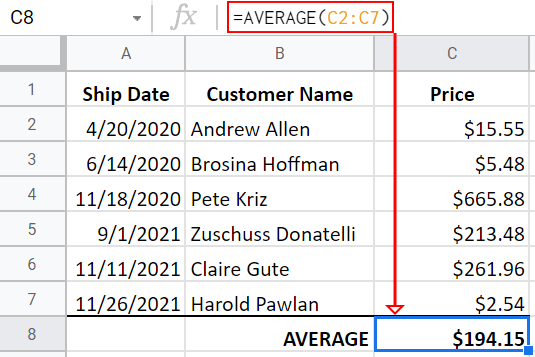
In this simple example, we compute the average of the item values ordered by customers from C2 through C7. The calculation is the same as adding the values and dividing by six.
Example 2 – AVERAGE When Some Values are Blank

The two Items Ordered columns above have the same total number of items. However, the 0s in column C are represented by actual zeros while rows 3 and 6 are blank in column D. AVERAGE only considers values that are not blank and are numerical. The function treats 0 as a number, and the AVERAGE function counts it, while it leaves an empty value out of the numerator and denominator. Consequently, the calculation on the right did not use cells D3 and D6. These two cells are null values, meaning they’re blank. Ignoring these two cells increases the result of the function from 2 to 4.
What if we defined a range that did not contain any numerical values? What would be the output in such a scenario?
Example 3 – AVERAGE Function with Checkboxes

As you can see, all values in the range C2:C7 are checkboxes. Google Sheets treats checkboxes as boolean values. A checked box is TRUE, and an unchecked box is FALSE.
Formula in cell C9: =AVERAGE(C2:C7)
Formula in cell C10: =AVERAGEA(C2:C7)
Since AVERAGE ignores boolean values, the formula in cell C9 ignored all the values. Ignoring the values means that the sum of values is zero divided by the number of values which is also zero. Mathematically, 0/0 is undefined, hence the reason we are getting a #DIV/0 error. To work with non-numeric values in the calculation of the average, use the AVERAGEA function instead. In the example, AVERAGEA returns 0.83, which means that 83% of the boxes are checked.
Example 4 – AVERAGE Function with Text
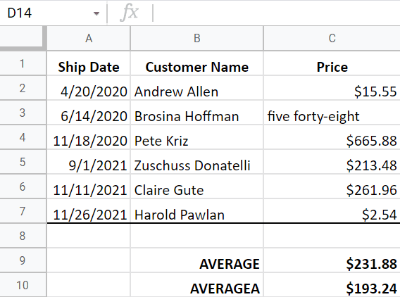
The formula in cell C9: =AVERAGE(C2:C7)
The formula in cell C10: =AVERAGEA(C2:C7)
Now our column of values, column C, has numbers and text. The treatment of the text in cell C3 makes a difference in this example. The AVERAGE function only uses the cells with numerical values. Therefore, AVERAGE is computing the average of cells C2 and C4:C7. AVERAGEA, on the other hand, counts text values as 0 and thus is using the entire range of C2:C7. The inclusion of cell C3 as a 0 significantly lowers the output.
Live Examples in Sheets
Go to this spreadsheet for examples of the AVERAGE and AVERAGEA functions shown above that you can study and use anywhere you would like.
Notes
- This function only uses numerical values.
- The AVERAGE function ignores blank cells and cells containing non-numerical values such as text and boolean.
- The AVERAGE function counts cells containing
0s since zero is a real number. - Consider using the SUBTOTAL function if you have multiple averages in one column.
Video Tutorials