SUBTOTAL deserves more attention than it gets. Despite its robustness, it is far less prevalent than functions such as SUM and AVERAGE. Let’s look at what you can do with this function in Google Sheets using this template to follow along.
Contents
Purpose
SUBTOTAL returns an aggregate result for a range of cells based on the specified function code.
Video Explanation
Syntax
=SUBTOTAL(function_code, range1, [range2,...])
Function codes:
range1– The first range for which to calculate the selected function.range2…– [OPTIONAL] Additional ranges to calculate the chosen function.function_code– The function to use for the aggregation.
The function code is a predefined constant representing what operation you wish to perform. You can apply any of the 11 operations within the functions listed above.
Alternative to SUBTOTAL
For an alternative method to deal with different levels of aggregation, spreadsheet.com enables the creation of row hierarchies, allowing you to nest levels of data to create parents, children, ancestors, and descendants. Read more about this feature to see if it could help you.
Example 1 – Summing a Range with Subtotals
There are many situations where the SUM function falls short, in which case the SUBTOTAL with a function code of 9 acts as a substitute. Let’s look at an example. If you had data containing subtotals for different categories and you wanted to find the total, you would have a few options at your disposal.
For example, you could use the + operator to add the cells one by one =cell1+cell2+cell3+... which could be tedious. Similarly, you could use the SUM function, which is susceptible to double counting. Instead, we could use SUBTOTAL to make the job much easier.
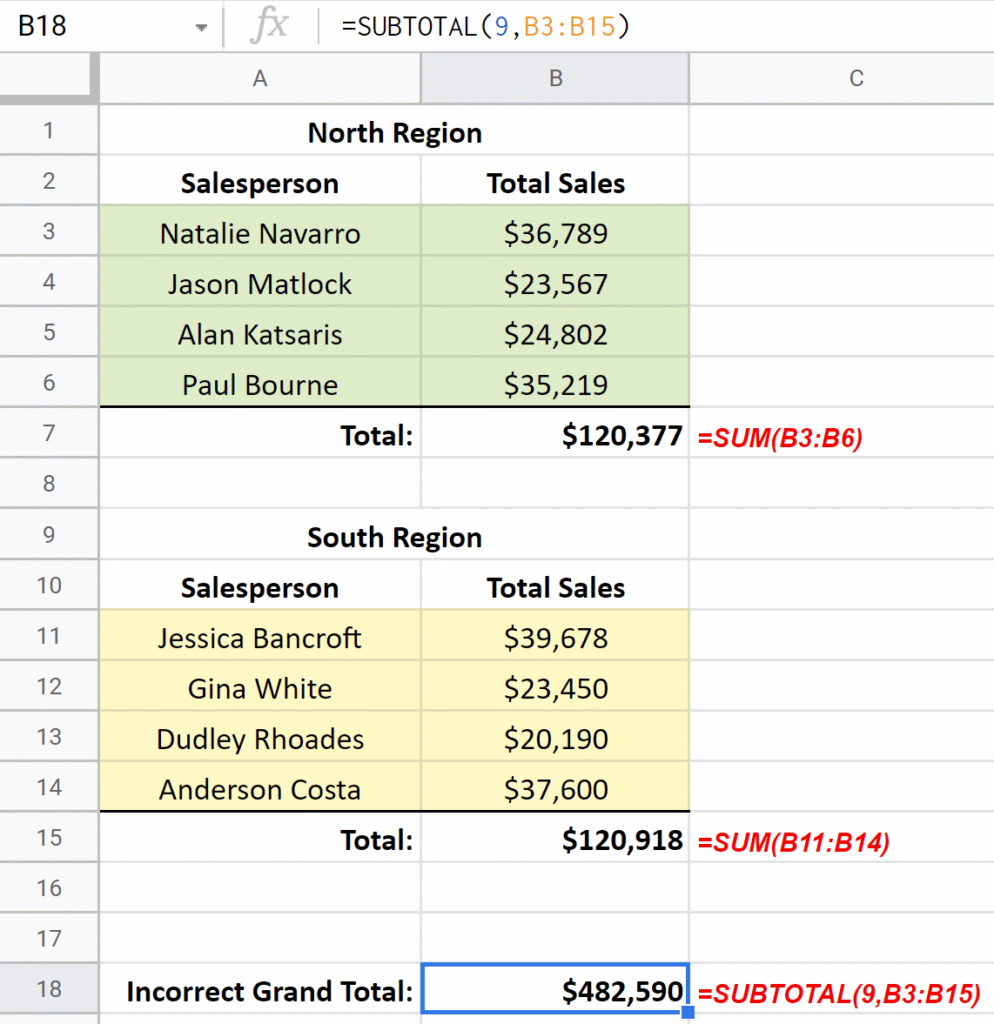
Our number of interest would be 9 because 9 corresponds to SUM. As a result, the formula would be =SUBTOTAL(9, range1, [range2],...). There is one caveat, however. You have to calculate the smaller totals first using the SUBTOTAL function. Take a look at the following dataset:

We can see that the above grand total in cell B18 is too large. SUBTOTAL adds all values in the specified range regardless of whether they are a total. This double-counting isn’t helpful to us and is quite similar to what the SUM function would do. How can we fix this?
We have to calculate the totals in cells B7 and B15 using the SUBTOTAL function with a function code of 9 so that the grand total will ignore these total cells. After making this switch, this is what we get:

Nice! The formula now gives us the correct total.
Example 2 – SUBTOTAL with Filtered Data
Using filters in your spreadsheet, the SUBTOTAL function will treat the filtered data differently than the underlying function, such as AVERAGE. The AVERAGE function will include filtered rows in its calculation.

The SUBTOTAL function will exclude filtered data using only the visible rows after filters are applied. You can see this difference below because AVERAGE is still returning $30,162 while SUBTOTAL with the function code 1 is returning $37,322.

Note that AVERAGE is one of the eleven functions available, and this different treatment of filtered cells occurs for all eleven.
Example 3 – Treatment of Hidden Rows
While example 2 dealt with filtered rows, a spreadsheet user can also hide selected rows. You can hide rows by right-clicking on the desired rows and choosing the Hide rows menu option.
Illustrating how the function treats hidden rows, this third example will use function codes 4 and 104. These codes call the MAX function, which returns the highest value in a data set. 4 will include the values in hidden rows and 104 will exclude them. In the first image, both function codes, 4 and 104, return the highest number in the range of $39,60.

While the image above shows all rows, the table in the picture below has row 9 hidden. Row 9 is also the row with the largest sales amount in the table. Therefore, function code 104 returns $37,600 as the maximum amount instead of $39,678 because 104 instructs the spreadsheet to exclude row 9 from its output.

Conclusion
As you can tell in the preceding examples and this template, the SUBTOTAL function provides flexibility and additional capabilities that other functions do not.
