
A mileage log answers “how far did I drive each day?” A report answers different questions: how many miles for each client, how many in March, how many for the second office. A pivot table gives you those answers from the same list without re-typing anything.
The steps below work on any list of drives with a date, a name and a distance. If your list comes from Calendar Mapper, its Trips tab is already laid out this way.
What your data should look like
A pivot table wants one row per drive and one value per column. Mixed rows, such as subtotals in the middle of the data, produce wrong totals. The Trips tab that Calendar Mapper adds next to the mileage log has exactly this shape:
- Date, Weekday and Month, so you can group by time
- Drive Type, Event Title, Origin and Destination, so you can group by who or where
- Distance, and optionally Time in Minutes, as plain numbers you can sum
The headers are on row 3, below a short banner, with a blank row 2 between them. Leave that blank row. It keeps Sheets from treating the banner as part of the headers.
Build the pivot table
- On the Trips tab, select the headers and data: click cell A3, then drag to the last column and row of the list.
- Choose Insert > Pivot table, keep New sheet, and click Create.
- Next to Rows, click Add and choose Event Title for miles per client or job. Choose Month instead for miles per month, or Destination for miles per place.
- Next to Values, click Add and choose Distance (mi). It sums by default.
- Widen column A so the labels read in full.
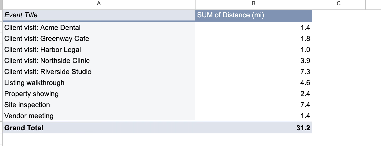
Add a second Rows field to nest the report, for example Month, then Event Title. Add Time in Minutes as a second value to see drive time next to miles.
Keep it working after the next import
Calendar Mapper clears and rewrites the Trips tab on every import. That is what keeps it matching the log, and it has two consequences:
- Put your pivot table, and any formulas, on their own tab. Do not add columns to the Trips tab; the next import will remove them.
- Select the whole columns for the pivot’s data range, for example
'Sheet1 Trips'!A3:I, so new rows are included when the list grows.
A check that catches mistakes
The pivot’s grand total should equal the total at the top of the mileage log for the same dates. If it does not, either the pivot’s range is too short, or you deleted or edited rows in one of the two tabs. Re-import rather than patching the numbers.
Going further
- A calculated field can turn miles into a dollar amount: multiply Distance by the current rate.
- To see which weekdays you drive most, group by Weekday, or use SUMIF by day of the week.
- For the rates and the records that go with the totals, see What a mileage log needs to include.
New to building the log? Start with How to make a mileage log from Google Calendar.