
This Google Sheets tutorial details two methods to total transaction values by day of the week. We’ll explore the versatility of the QUERY function and delve into the power of Pivot Tables to create these summaries.
Make a copy of this live Google Sheet to follow along. Adjust the directions accordingly when using your data.
Contents
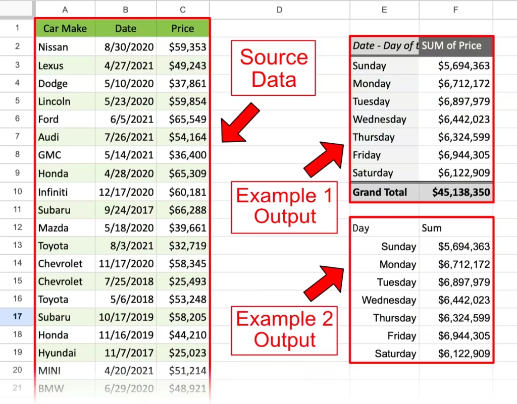
Desired Outcome
First, let’s define our goal. We want to find totals for each day of the week from a list of transactions on multiple days. The output will be a list of each day next to its corresponding total.
Now, let’s start with the first solution. If you’re not a fan of long formulas, this will be the one for you.
💡 Pro Tip – Use the Calendar Importer add-on to bring dates in directly from Google Calendar.
Example 1 – Pivot Table with Date Grouping
This first example will use the built-in date grouping feature for pivot tables in Google Sheets. This feature will do most of the work for you, eliminating the need for formulas.
Pivot tables summarize large amounts of data using menus instead of formulas. See this YouTube video for a primer on pivot tables if you are unfamiliar with them.
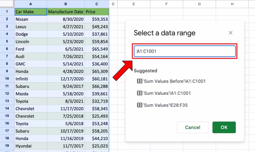
Start by going to the Insert menu, then choosing pivot table. Specify A1:C1001 as the data range.
Press OK once you have the correct data range.
Native pivot tables can have only one data range. Use OmniPivot if you have more than one range.

Then Google Sheets will ask where you want the Pivot table.
We’ll place it on the Existing sheet in cell E2. Choose the location and click Create.
Clicking the Create button brings up the Pivot table editor in the sidebar. In the editor, we’ll drag and drop the Manufacture Date field into the Rows and the Price field into the Values.

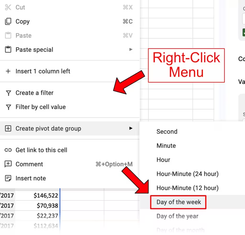
Then, right-click on the dates, choose Create pivot date group, and select Day of the week.
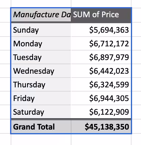
Now, you have a finished pivot table with the amounts summed by day of the week.
As you can see, pivot tables do much of the work without code. However, the query function is best if you want to use a formula and have more flexibility. Let’s look at that now.
Example 2 – Query Function
The query function is in a class of its own compared to traditional spreadsheet functions. It allows the spreadsheet user to write SQL commands inside the formula. We’ll use query to sum the amounts by day, just as we did above, but with one formula. Let’s take a look at the query syntax.
Query Function Syntax
=QUERY(data, query, [headers])
data– Location of the dataquery– The query statement. The query is composed of optional clauses that you must use in order.select– The columns to return. If omitted, the query returns all columns.where– Conditions that rows must meet- group by – Aggregates values
pivot– Aggregates values into new columnsorder by– Sorts rows by valueslimit– Limits the number of rows returnedoffset– Skips a specified number of rowslabel– Creates column labelsformat– Formats outputsoptions– Sets additional options
[headers]– The number of header rows at the top of thedata
Writing the Query
Now that we know the syntax let’s write out the formula. We will still use A1:C1001 as the range and there’s one header row. So, we know the values for the data and headers arguments. Here is what we have so far:
=QUERY(A1:C1001, query, 1)
For the query, we want to return a column for the day of the week and a column for the sums. SQL has a scalar function called dayOfWeek and an aggregation function called sum. We’ll use both of those. We’ll then use the group by clause to tell the function how to show the output, and we’ll add headers using the label clause. To polish it off, we’ll use the format clause to change the day numbers to words and the numbers to currency. This is what the formula looks like now:
=QUERY(A1:C1001, "select dayOfWeek(Col2), sum(Col3) group by dayOfWeek(Col2) label dayOfWeek(Col2)'Day',sum(Col3)'Sum' format dayOfWeek(Col2)'dddd',sum(Col3)'$#,##0'", 1)
Breakdown of the QUERY Function
dayOfWeek(Col2) | Converts the date to a day number (1-7) |
Group By | Groups the rows based on the specific day |
Format | Changes the day number (e.g., 1) to the day name (e.g., Sunday) |
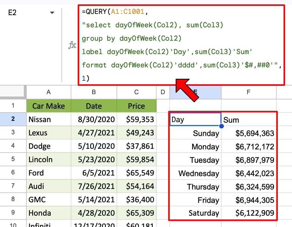
The long formula creates this simple, compact table of just the data you need, sorted by day of the week!
Video Tutorials
Conclusion
Google Sheets has two great options for summing data by day of the week. Choose the pivot table for ease of use and the query function for the power of a formula written in SQL. Whichever technique you use, you’ll get the answer you’re looking for.
Related Tutorials
-
Show the Day of the Week as Text – Google Sheets
This tutorial shows you two ways to display your dates as the day of the week in your spreadsheet. The default is to show the month, day, and year together. Therefore, you will have to make a few changes depending on the type of output you want. Grab a copy of this template to follow…
-
Sum Amounts for Each Day of the Week in Google Sheets
Learn two techniques to sum values by day of the week.
-
Types of Date and Time Functions in Google Sheets
The date and time functions in Google Sheets can be grouped into different categories based on their purpose.