The SUMIF function is used in Google Sheets to add numbers if data meets a specific condition.
Use SUMIFS to check for multiple conditions. Feel free to copy the template with these examples to follow along.
Purpose
This function returns the total of a series of numbers, cells, or both that meet a specific condition.
Syntax
SUMIF(range, criterion, [sum_range])
range– The range with the criterion.criterion– The condition that must be TRUE to sum.sum_range– The range for the function to sum. Only used if thesum_rangeis different from therange.
Related Functions
IF – Returns a value based on a condition.
SUM – Add numbers regardless of their value
SUMIFS – Adds numbers based on multiple criteria
Video Tutorial
Common Error
#REF! – One cause is a circular dependency created by overlapping a range with the function’s cell.
Examples
Example 1 – Sum Values Greater Than or Equal to an Amount
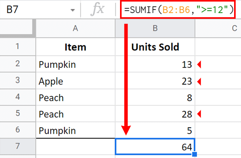
Let’s say that you are tracking orders of produce from a warehouse. Every order of twelve or more items requires a container. You wonder how many items you will be packing today.

You can calculate the total Items to pack using the formula =SUMIF(B2:B6,">=12") shown in the image above. Notice the quotes around ">=12". Even though 12 is not a text value, the SUMIF function requires quotes around the condition. Typically quotes are used in spreadsheet formulas when referring to text. Read more about this inconsistency here.
How would we do this if we wanted to know how many peaches our customers ordered?
Example 2 – Sum Values When a Word Matches
Now let’s find the total number of preaches sold.

When matching a text value, you will always need to use the column you are evaluating first, then the criterion, then the range to sum. In the case shown in the image above, we look for Peach in A2:A6. Then, we sum the values in B2:B6 for each row with the word Peach. The formula is =SUMIF(A2:A6,"Peach",B2:B6). This formula adds the values 8 and 28, resulting in 36.
Example 3 – Sum Values Before a Certain Date
Now things get more complicated with this function. Using dates and times can be tricky, but this function makes it even more complex, as shown next with the formula’s required use of the &.

As seen in the image above, you need to split the < from the date with an &. Once you get this part down, the rest is easy. This formula looks at the range A2:A6 to decide if it should sum the amounts in C2:C6 based on their date.
Example 4 – Sum Values with Partial Matches
You only need to match some letters in a cell for your condition.

In this example, we evaluate the words in A2:A6 for any that start with the text Pumpkin. The * is a wildcard that can represent any character or multiple characters. The other two wildcards available are ?, which is one of any character, and ~ which escapes the * and the ? if you want to use them as non-wildcards.
Examples in a Live Template
See this template for a spreadsheet with the examples used in this blog. You can make your own copy and use them in your work.
