The ARRAYFORMULA function is a powerful tool in Google Sheets that allows you to spread formula outputs across multiple rows and columns. It can extend non-array functions such as SUM, PRODUCT, or AVERAGE.
As with other functions that generate arrays, such as FILTER and QUERY, the output needs space to expand below and right. Keep this in mind so you do not overwrite other data.
💡 Use the shortcut key combination of Ctrl+Shift+Enter to wrap your function inside ARRAYFORMULA.
Syntax
=ARRAYFORMULA(array_formula)
arrayformula– Can be one of the following:- A cell range
- Mathematical expression with ranges of the same size
- A function returning multiple cells
Related Functions
ARRAY_CONSTRAIN – Limits array output
QUERY – Performs SQL-like complex array operations
SUMPRODUCT – Calculates the sum of multiplied range values. Consider this function instead if you are using the ARRAYFUNCTION for multiplication.
Important Considerations
- ARRAYFORMULA requires sufficient space below and to the right of the formula to expand its output.
- Ensure input ranges are of equal size to prevent errors.
- The formula automatically adjusts when rows are added or deleted.
Video Tutorial
Examples

The table pictured above is the source data used for all the examples. It represents a company’s inventory consisting of different types of items, number of cases, number of items per case, and location.
Example 1 – Simple Column Replication
The formula in the top cell is =ARRAYFORMULA(A1:A13).

The formula copies an entire column without modifying the source data in A1:A13. This can be useful for duplicating data while keeping the original intact.
When you update the source data, the output updates automatically.
Example 2 – Return a Row
The formula in the left cell is =ARRAYFORMULA(A2:D2).

The ARRAYFORMULA also produces horizontal array output. This showcases versatility across rows and columns.
Example 3 – Multiplied Column
The formula in cell E2 =ARRAYFORMULA((B2:B13)*(C2:C13))

Using the ARRAYFORMULA to extend multiplication down a column is an excellent example of the power of this function. This formula repeats a multiplication formula 12 times, once in each row. If you delete rows from the table, the formula will automatically adjust.
Note that each range in the input needs to be the same size. In this example, the ranges of B2:B13 and C2:C13 both span 12 rows. If you have a very long table, you could drop the ending row values, such as B2:B and C2:C. Removing the ending row numbers would extend the formula to the bottom of the spreadsheet.
Example 4 – Conditional Multiplication
The formula in cell E2 is =ARRAYFORMULA(IF(D2:D13="North",(B2:B13)*(C2:C13),0)).

The ARRAYFORMULA can perform complex data filtering. The formula used for the array_formula input can be more complex if needed. In this case, we have added an IF statement to limit the multiplication to only the North warehouse.
Example 5 – Text Concatentation
The formula in the top row is
=ARRAYFORMULA("The "&D2:D13&" warehouse has "&B2:B13&" cases of "&A2:A13&"s.").

In this example, we use it to combine text and numeric data dynamically. The automatically creates descriptive phrases. Using the & sign is similar to the CONCATENATE formula.
Example 6 – Multidimensional Arrays
For this last example, we will use a different data set.

Previously, we looked at how arrays can be vertical or horizontal. They can also be multi-dimensional.
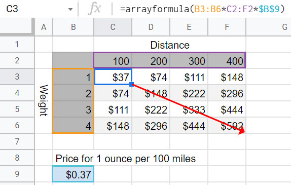
This table calculates shipping rates. The formula, =ARRAYFORMULA(B3:B6*C2:F2*$B$9), is multiplying the range of B3:B6 containing the Weight, the range of C2:F2 containing the Distance, and the Price for 1 ounce per 100 miles in cell B9. Notice that the $s in B9 are fixing the row and column references to stay the same in every cell. The array formula multiplies the three values and writes its results below and to the right.
Live Example in Sheets
Go to this spreadsheet for examples of the ARRAYFORMULA function shown above that you can study and use anywhere you want.

