Spreadsheets users often need to hide data in their spreadsheets. Let’s say you have a file with employee pay details, and only personnel in the human resources department are allowed to see it. However, the accounting department needs to access summarized data.
We will walk through a scenario where one user can see the detail while another can only see the summary. We will accomplish this by creating connected spreadsheets and controlling the permissions on each.
ℹ️ You could implement a similar permission structure at the department level using Shared Drives, a feature available in Google Workspace.
Contents
Video Tutorial
Confidential Data
This spreadsheet holds confidential data.

At this time, there is only one worksheet in this file named Detail. You are the file owner, and you are sure that you have not granted permissions to other users. We will create a new sheet with summary data for the accounting department.
Create a Summary Sheet
The first step in this process is to add a new sheet to this file.
Click the + sign to add a new sheet and rename it Summary. After adding the new sheet, we are ready to use it for the summary data we create in the next step.
Add Summary Data to the New Sheet
Now we have a blank sheet called Summary where we can create the data to be shared.

Create a Pivot Table
We want to aggregate the Detail sheet in the Summary sheet in a way that does not reveal any employee names. The easiest way to accomplish this is a Pivot Table. Go to the Insert menu and choose Pivot table.

Once you have chosen inserted a pivot table from the menu, you get a pop-up with several fields.

The Data range for the pivot table is in columns A through E of the other worksheet. You can select that range with your mouse or type Detail!A:E. As a result of leaving the row numbers off, the formula captures any new rows. We created the Summary sheet for this table, so you can use the Existing sheet option and place it in cell B4 of this sheet shown by typing Summary!B4. In this case, you don’t need to type the Summary! before B4 since you are not referencing another sheet, you can leave it if you want.

Populate the Pivot Table
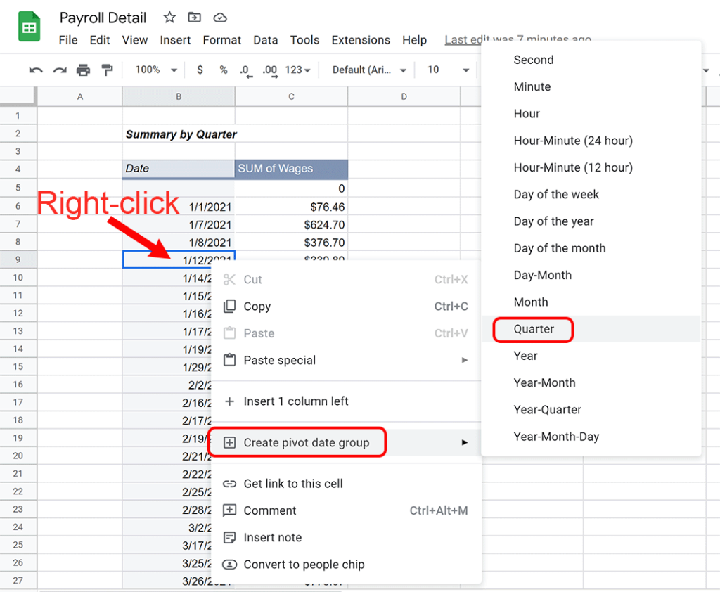
We want the pivot table to have Wages as the Values and the Date values as the Row labels. Additionally, we want to summarize the dates by quarter. Let’s do that next.

Summarize the Pivot Table by Quarter
There is one more issue to deal with before we use IMPORTRANGE. The pivot table has an ugly blank row with a zero total. This blank row is from the empty rows we picked up using cell references with no row numbers for the Date range.

However, we can quickly remove the row with zeroes by adding a filter to remove all zero values.
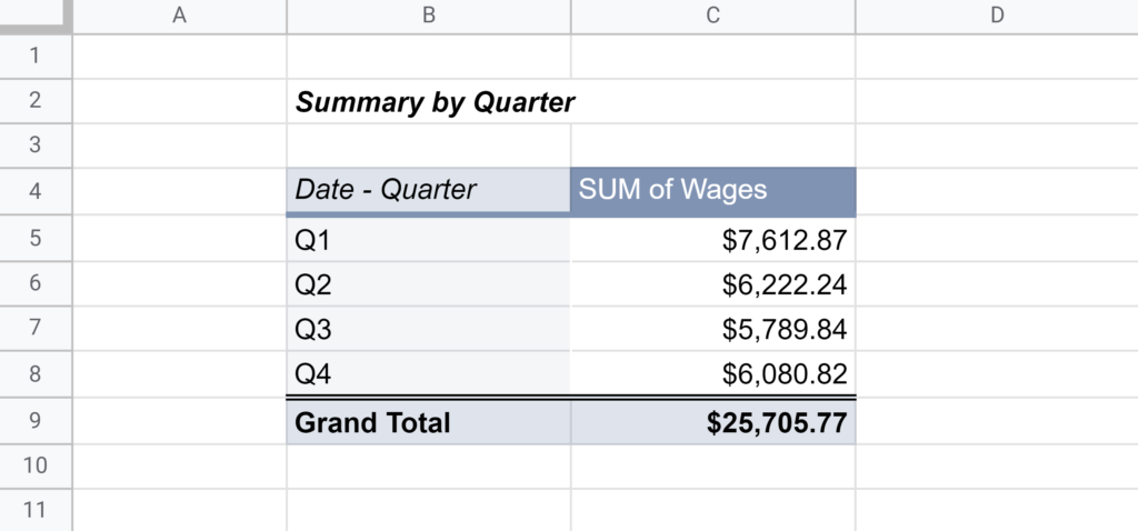
As a result, we have a clean pivot table without the blank row at the top.

This table now contains summary data for the accounting department without revealing names. However, the Detail sheet still contains confidential data. This brings us to the next step of this tutorial, where we will bring this summary data into a separate file.
Create a New Spreadsheet to Hide Data
We will create a new spreadsheet to import the summarized data.

As a result, this new spreadsheet can be shared with your coworker in the accounting department as it does not contain confidential data.

After adding another user to the new spreadsheet, you can bring in the protected data from the source spreadsheet. We will use IMPORTRANGE for this.
Use IMPORTRANGE
IMPORTRANGE brings data from one spreadsheet into another. We will use it to get the payroll summary data into a new spreadsheet while leaving the detail in the source spreadsheet.
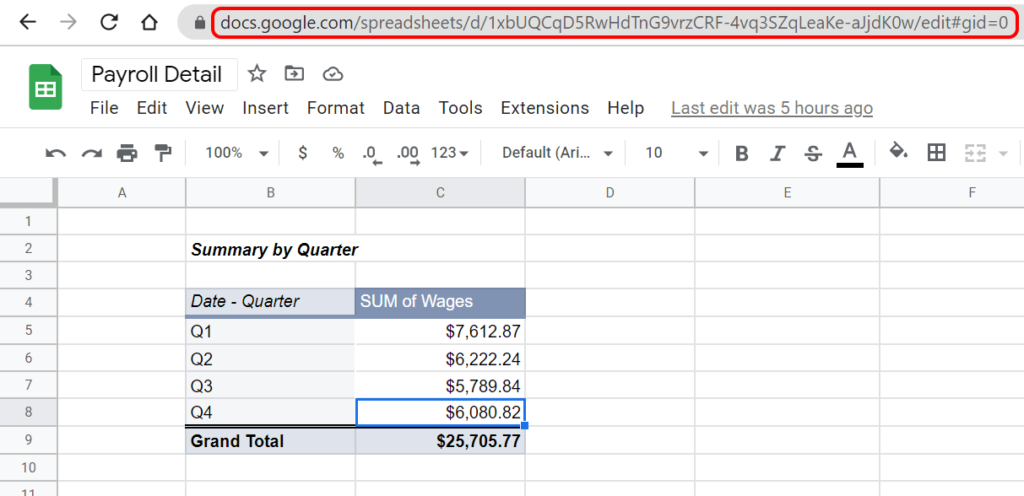
The IMPORTRANGE’s first input is the spreadsheet_url of the source spreadsheet. This URL is the web address of the spreadsheet with the original data.

The second input for IMPORTRANGE is the range_string. This string is the cell reference in the source spreadsheet. Putting these two items together, we have the following formula: =IMPORTRANGE("1xbUQCqD5RwHdTnG9vrzCRF-4vq3SZqLeaKe-aJjdK0w","B4:C9"). We only used the middle portion of the spreadsheet_url between d/ and /edit called the spreadsheet key. You may use the entire URL if you want.
After entering the formula, you will get a #REF! error until you click the button to allow access to the other sheet.

After you allow access, the data comes into the new spreadsheet.

At this point, the payroll summary is almost finished. You have brought in the appropriate data, and the users cannot see anything confidential. However, remember that IMPORTRANGE has given all owners of this new spreadsheet access to the other sheet with the hidden data. Someone could change the data_range of the function to pull in more cells. The user would need to append the other worksheet name onto the cell reference in our example. Changing the cell reference is unlikely but possible. However, using a long, random name for any worksheets containing sensitive data is an extra step that you could take if desired.

In conclusion, you should now be able to connect two Google Sheets with different permissions to hide data from certain spreadsheet users!
