
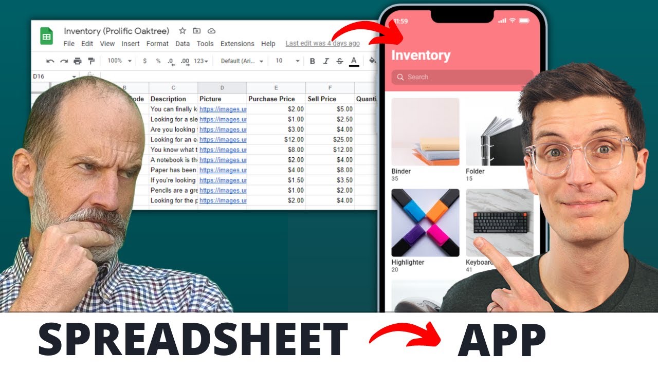
This tutorial focuses on three must-know Google Sheets functions for building a no-code app. No-code app builders may not be familiar with spreadsheets, just as spreadsheet users (gulp) may not know how to build an app. I had the pleasure of working with Darren Alderman, who makes Glide apps for Google Sheets. We collaborated on a YouTube video and the article below to bring you this guide.

The three functions will connect and summarize four spreadsheets. We will focus on quickly deploying repeated functions with ARRAYFORMULA, connecting spreadsheets with IMPORTRANGE, and arranging that data with the versatile QUERY function.
Before we start, you can grab a copy of the main spreadsheet and the four spreadsheets (North, South, East, West) that connect to it. You must copy them into your Drive for the IMPORTRANGE functions to work.
Contents
YouTube Video
Use IMPORTRANGE to Connect Spreadsheets
The first function no-code app developers can use is IMPORTRANGE. This function brings data from one spreadsheet into another. In this case, we will use four IMPORTRANGE functions to fetch data from the North, South, East, and West spreadsheets to summarize in a destination spreadsheet.

We will build the functions in the Combined Sales spreadsheet. First, we’ll create the IMPORTRANGE function to connect to the North Sales spreadsheet. IMPORTRANGE needs two inputs to work – the spreadsheet_url and range_string. Go to the North Sales spreadsheet and copy its web address for the spreadsheet_url.

We will use this address in the first of four connections. We’ll go back to the Combined Sales file and complete the first formula.

The formula, using the spreadsheet_url from the North Sales spreadsheet, is as follows:
=IMPORTRANGE("https://docs.google.com/spreadsheets/d/1m5DUaLAxLwE_PYQ-t2qfAkQq1yrtw9UvEYpInJ-Yy6Q/edit#gid=0","A1")
Once you enter the formula, you will get a #REF! error. If you click in the cell, you will see a blue button you must click for the spreadsheet to connect. Notice we are just using A1 as the range_string. At this point, we just want to get access to the other spreadsheets. We will be pulling in more data with QUERY later in this tutorial.

Now repeat this process, writing the formula to allow access to the other three spreadsheets.

Cell A1 in all four spreadsheets contains the text value Construction Material. We know the functions are working since you see these values in the destination spreadsheet. Now that we have the functions working let’s prepare the other spreadsheets.
Use ARRAYFORMULA to Repeat Functions
Each row in the source spreadsheets needs to have a Total column. This total will be Quantity * Price. However, we need to multiply forty rows between the four spreadsheets. Instead of repeating the multiplication formula forty times, we will use the ARRAYFORMULA once in each spreadsheet.

The formula =ARRAYFORMULA(B2:B*C2:C) is only in cell E2. This formula fills the cells below E2.
There are two items to take note of. First is the lack of ending row numbers on the two cell references of B2:B and C2:C. Secondly, the zeros you see in column E starting in row 12. We built the ARRAYFORMULA with no bottom row, so it includes any new rows added later. For example, if we added numbers to cells B12 and C12, the product would appear in E12.
Now add the ARRAYFORMULA to the other three source spreadsheets. After adding the formulas, we are ready to bring the files together in Combined Sales.
Setting up QUERY for your No-Code App
There are a few items to take care of before diving into the QUERY function.
Spreadsheet Keys
First, let’s set up the four spreadsheet_urls for the QUERY function’s reference. Instead of using the full web address of each spreadsheet, we can use the random string of characters in the middle of the URL called the spreadsheet key. Copy them from the four URLs and paste them into cells.

Now that we have the spreadsheet keys let’s make them easy to reference.
Named Ranges
The destination spreadsheet has a worksheet named Set Up and a worksheet named Query. Since our QUERY will be on a separate worksheet from the spreadsheet keys, pulling the spreadsheet keys into the Query worksheet requires a long reference like 'Set Up'!A1. Let’s name the four cells with the spreadsheet keys to avoid these long names.

Now we can refer to cell C11 as North instead of 'Set Up'!C11.
Writing the QUERY
Now that we’ve named the spreadsheet keys’ ranges, we are ready to write our QUERY. The purpose of the QUERY is to bring in the data from the four spreadsheets for use in your no-code app.
We will be using IMPORTRANGE functions inside of the query. You have to grant permissions to the IMPORTRANGES before using them in a query which is why we performed those steps earlier in this tutorial. We will put the IMPORTRANGEs inside curly braces ({}) to indicate they are creating an array and separate them with semi-colons to indicate that they vertically stack. Note that only the North spreadsheet range starts at row 1 (A1:E). Staring at row 1 only once avoids duplicating the header row.
=QUERY( {IMPORTRANGE(North,"A1:E"); IMPORTRANGE(West,"A2:E"); IMPORTRANGE(East,"A2:E"); IMPORTRANGE(South,"A2:E") }, "select *",1)
This QUERY function gets us pretty close to what we want.

However, notice the zeroes at the bottom. The zeroes extend to row 1000 before the data from the West spreadsheet starts. Remember when we dropped the ending row from the ARRAYFORMULAs? The query is pulling in those extra rows. Let’s tell it not to. We will add where Col1 is not null onto the QUERY, stopping it from pulling in rows with empty cells in column A.
ℹ️ The QUERY needs to refer to A as Col1 when working with multiple worksheets.
=QUERY( {IMPORTRANGE(North,"A1:E"); IMPORTRANGE(West,"A2:E"); IMPORTRANGE(East,"A2:E"); IMPORTRANGE(South,"A2:E") }, "select * where Col1 is not null",1)
Now you have one consolidate table.
Ready for your No-Code App
Knowing how to add repeating functions with ARRAYFORMULA, bring other data in with IMPORTRANGE, then summarize it all with QUERY are three things that will enable you to use Google Sheets for your no-code app like a pro!