The IFS function in Google Sheets evaluates multiple conditions and returns a value based on the first true condition. It is a logical function that works similarly to the IF function but can handle more than one condition.
The IFS function evaluates the conditions individually, starting from the first one. If a condition is true, the function returns the corresponding value and stops evaluating the remaining conditions. This function returns an #N/A error if no conditions are met, unlike the IF function, which can return an alternate value if a condition is not met. See example 3 to work around this limitation.
Contents
Syntax
=IFS(condition1, value1, [condition2, value2], ...)
condition1– The first condition evaluatedvalue1– The value returned if the first condition is true[condition2, value2], [condition3, value3], ...– Optional additional conditions and values
Similar Functions
IF – Return one value if TRUE and another if FALSE
COUNTIFS – Count cells that match multiple criteria
SUMIFS – Sum values that match multiple criteria
COUNTUNIQUEIFS – Count unique values that meet multiple criteria
Example 1 – Assigning Letter Grades
First, let’s use the IFS function with multiple conditions to calculate letter grades.

=IFS(B2>0.9,"A",B2>0.8,"B",B2>0.7,"C",B2>0.6,"D",B2<=0.6,"F")
In this example, if the value in cell B2 is greater than 90%, the function returns “A“. If it is greater than 80% but less than or equal to 90%, it returns “B“, and so on. If the value in cell B2 is less than or equal to 60%, the function returns “F“.
Example 2 – Using IFS to Add Symbols
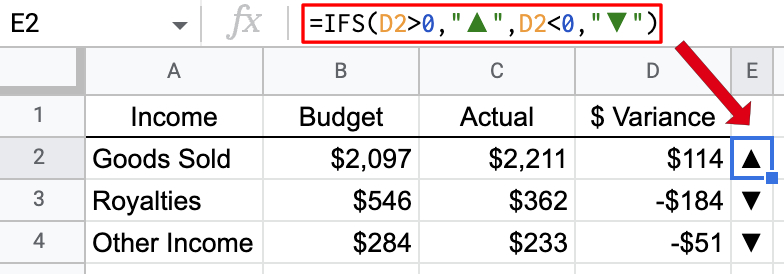
Here’s an example of how to use the IFS function to insert special characters.

Formula used in cell E2: =IFS(D2>0,"▲",D2<0,"▼")
In this example, we use upward and downward-facing triangles to indicate trends. If the $ Variance is positive, we use a triangle pointing up, and if the $ Variance is negative, we place a triangle pointing down.
You can use the Insert Special Characters add-on to place the triangles in your sheet without leaving the Google Sheets app.
Example 3 – Avoiding an Error
Lastly, let’s look at how to handle the #N/A “No match.” error. In this example, the IFS statement knows which Rep to assign for High and Medium Severities, but there are no Reps designated for other Severities.

Formula used in cell B2: =IFS(A2="High","Rick",A2="Medium","Marge")
For cell B2 above, the function goes through the two conditions, and both evaluate to FALSE. To handle situations such as these, we’ll add a TRUE condition to the end to satisfy any other values.

Formula used: =IFS(A2="High","Rick",A2="Medium","Marge",TRUE,"Open ticket")
Now any value other than High or Medium will return “Open ticket.”
Live Template
See this template for a spreadsheet with the examples used in this article. You can make your copy and use them in your work.
Video Tutorial
Conclusion
The IFS function is both powerful and flexible when used properly. Leave us a comment below if you have any questions or suggestions for different uses.
