Rating chips in Google Sheets are a great way to collect data and feedback from others. They are one of several Smart Chips that extend a cell’s ability to store data. In this article, we’ll show how three friends rated their dinner experience at a new restaurant using Rating Chips.
The three friends, Jean, Bob, and Dwayne, had dinner at a newly opened, fancy restaurant. They were excited to try the food and see the atmosphere.
Contents
Setting up the Google Sheet
After dinner, they decide to use Google Sheets to rate their experience. They create a new spreadsheet and share it with each other. They add a column for each friend and a row for each rating category, such as Service, Value, and Food.
💡 Follow along with a copy of the spreadsheet as we work through the example.

Inserting the Rating Chips
After setting it up, this spreadsheet has a good space for the Rating Chips in the cell range of B2:D4. Now, let’s select that range and insert the Ratings Chips.

To insert a rating chip:
- Select the cell(s) where you want to insert the rating chip.
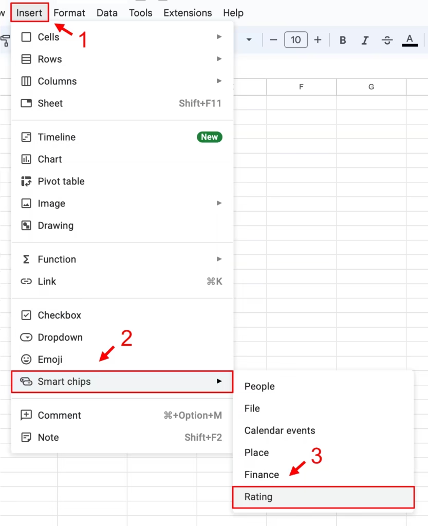
- Click Insert > Smart chips > Rating.

Giving the Star Ratings
Jean, Bob, and Dwayne each rate the restaurant’s service, value, and food. To change the number of stars, they can click on each star and select how many they want, or type a whole number between 0 and 5.
Once they’ve rated each aspect of the dining experience, they can use Google Sheets to calculate the average rating for each.
Calculating the Average Rating
Before writing the formula for calculating the average, it is important to understand that Rating Chips represent whole numbers from 0 to 5. Next, use the ROUND function to eliminate any fractional values. Let’s write our first formula in the row with the Service ratings. This cell reference will be B2:D2.
- Start your formula with the
=sign. - Then, write out the ROUND function and give it the AVERAGE function as its argument.
- Then, give the average function the cell range.
- The formula will be as follows:
=ROUND(AVERAGE(B2:D2))

Copy and paste this formula into the next two rows.

The average rating for the Service is 4 stars, the average rating for the Value is 4 stars, and the average rating for the Food is 5 stars.
Video Tutorial
Conclusion
Using rating chips in Google Sheets is a great way to collect data and feedback from others. It’s also a fun and interactive way to share your experiences with friends.
Related Articles
-
Calendar Mapper – Mileage Logs from Google Calendar
Your appointments are already in your calendar. Now let your mileage log write itself. Calendar Mapper imports your Google Calendar events into Google Sheets and calculates the miles between each stop — so every client visit, every commute, and every deduction is accounted for. “Every client visit, every commute, every deduction — your calendar remembers…
-
How to Use Place Chips in Google Sheets
Learn about Place Chips and how to use them in Google Sheets.