
This tutorial presents several methods for counting unique values in Google Sheets based on meeting certain conditions.
We will go through these examples using a beginner technique with built-in functions, an intermediate method using pivot tables, and a pro-level technique using the QUERY function in Google sheets.
Contents
Source Data
We will use the warehouse inventory data listed below for all the examples.

You can get a copy of the spreadsheet with this data and the examples. If using your spreadsheet, make sure your columns contain similar data and there are no extra spaces or capitalization differences that may throw off the analysis.
Beginner-Level | Built-In Functions
These beginner examples are the easiest to implement because they use familiar-looking spreadsheet functions. Although the functions may be new to you, their usage and syntax are similar to more common functions such as SUMIF and COUNTIFS.
Let’s start with the first question that we’ll be answering.
How Many Unique Items are at Each Warehouse?
The first question is how many different types of items are at each of the three warehouses. It is important to note that we are not looking for total items. For example, five hammers and three saws are two unique items.
We want the first column to be the warehouses, so let’s make that column first.
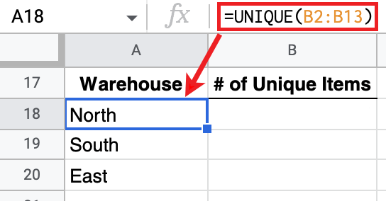
The UNIQUE function is the perfect choice to list the warehouses. It searches through the twelve values in B2:B13 and returns one instance of each distinct value. In this case, one of each of the three warehouse locations – North, South, and East. The formula =UNIQUE(B2:B13) resides in cell A18, but its output fills the three cells in A18:A20.
Now we’ll bring in the awkwardly named COUNTUNIQUEIFS function, which, as you can guess, is more complex.

Formula used: =COUNTUNIQUEIFS(A$2:A$13,B$2:B$13,A18)
This formula’s first argument is the range to be counted. We want to count the Items which are in A2:A13. Since COUNTUNIQUEIFS cannot produce an array like the UNIQUE function, copy this formula from B18 into B19 and B20. However, you don’t want the row numbers to change when you copy and paste. Therefore, use $s to change the row numbers from relative to fixed. These $s change the range reference from A2:A13 to A$2:A$13.
The second argument in the formula is criteria_range of B$2:B$13 which is the Warehouses. This is the range that will be tested against the third argument, which is the criterion in A18.
The completed functions tell us there are 4 different items at the North warehouse, 3 at the South warehouse, and 2 at the East warehouse.
How Many Warehouses Have Each Item?
Let’s run through another example using the UNIQUE function together with the COUNTUNIQUE function. This time, we will flip the question and look at the number of Warehouses instead of Items. Accordingly, let’s make the first column Items.

We see the power of the UNIQUE function at work again as the formula =UNIQUE(A2:A13) generates six values from one function. There is no need to fix the row number inside the formula since the function does all of its work from one cell.
Next, we’ll use the COUNTUNIQUEIFS formula, but we’ll switch the inputs.

Formula used: =COUNTUNIQUEIFS(B$2:B$13,A$2:A$13,A27)
We will switch the range to the Warehouses which are in B2:B13 of the inventory listing. Remember to fix the rows with $s again to keep the row numbers from changing when you copy the formula into the subsequent rows.
The second and third arguments in the formula are the criteria_range to be tested, A$2:A$13 and the criterion in A27. By listing the criteria with the UNIQUE function and then referencing them, we ensure there are no typos and we don’t miss any items.
The resultant list tells us how many warehouses carry each type of Item. For example, Wrenches are stocked at the North and South warehouse. Even though there are two Wrenches at the North Warehouse (rows 2 and 10), the second listing of a Wrench is not a unique value.
How Many Warehouses Have More Than 10 Cases of an Item?
We’ll show the power of the COUNTUNIQUEIFS function by using two criteria for this last question. We’ll be asking how many warehouses have more than 10 cases of any items.
The first step is to use the UNIQUE function the same way we did in the second example – =UNIQUE(A2:A13).

Next, we’ll use the COUNTUNIQUEIFS function with two criteria and two criteria_ranges.

Formula used: =COUNTUNIQUEIFS(B$2:B$13,A$2:A$13,A39,C$2:C$13,">10")
This long formula is not as complex as it looks at first glance. The range is B2:B13, which contains the Warehouses to be counted.
Next, to count how many warehouses have more than 10 of each Item, our criteria_ranges are A2:A13 and C2:C13 as they contain types of Items and the number of Cases.
Using these formulas, we see 1 warehouse holding more than 10 wrenches, 1 holding more than 10 nails, and 2 holding more than 10 pairs of pliers.
We certainly got the answers we were looking for using the functions built-in to Google Sheets. However, pivot tables can provide a more flexible solution. Let’s look at these next.
Intermediate-Level | Pivot Tables
Pivot tables are a data analysis shortcut. Instead of writing functions, we use a graphical user interface to create reports. Let’s revisit the questions and answer them with Pivot tables.
First, let’s take another look at the source data.
This inventory listing is the same table of data we used previously in this tutorial.
How Many Unique Items are at Each Warehouse?
To start building your first pivot table, go to the Insert menu and choose Pivot table.
Select the source table for the Data range. Make sure you include the headers. In this case, we will use A1:C13. Notice that Google Sheets prepends the worksheet name to the cell reference. This prepending is optional as long you are working on only one sheet. However, you can leave the worksheet name on the cell reference, which will still work. Use the OmniPivot add-on if you have more than one Data range.
Let’s place the pivot table in cell D17. This location is where it fits in the example template.


It is easiest to build a pivot table by first adding the Values field. Since we want to see how many Items are at each Warehouse, add the Item field to the Values and change the Summarize by drop-down to COUNTUNIQUE.
We want the Warehouses listed in rows, so add the Warehouse field to the Rows area in the Pivot table editor. Now you’ve created your first table without using any functions.
The Pivot table provide the same correct answer as the built-in functions we used earlier.

How Many Warehouses Have Each Item?
You already know how to create a Pivot table, so we’ll move on to changing the Pivot table editor.
We want our output to have rows of Items on the left and unique counts of Warehouses to each Item‘s right. Therefore, we place the Warehouses in the Values and the Items in the Rows.

That was easy! Here is the finished table.

How Many Warehouses Have More Than 10 Cases of an Item?

Now let’s look at our last question with a pivot table. It won’t be too difficult to put together, but we will have to bring in another feature of Pivot tables. This feature is a Filter, similar to adding criteria to a function.
A filter blocks unwanted data from coming into a Pivot table. We don’t want to see warehouses with fewer than 10 cases, so that’s how we will set our filter.
After setting the filter, we have a Pivot table showing us the correct answer. Interestingly, the Items that don’t make it through the filter, such as the Hammers, aren’t shown with 0s. Instead, the filter leaves them out of the table.
Here is the finished Pivot table showing us how many warehouses contain more than 10 cases of each Item.

⚠️ Looking at the Pivot table output, you cannot tell if someone has applied a filter. Use a slicer if you want the filter to be noticeable.
Pro-Level | QUERY Function
When you’ve mastered “regular” functions and become a Pivot table expert, it’s time to learn the QUERY function. QUERY is the swiss army knife of Google Sheets’ spreadsheet functions.
QUERY brings the power of SQL to Google Sheets, allowing you to use this programming language’s expansive syntax. SQL is for database queries, so it is well-suited for spreadsheet data organized in a table.
Let’s use the QUERY function to answer the same three questions. We will use the same source data.
How Many Unique Items are at Each Warehouse?
We will answer this question with one, albeit large, query.
Formula used: =QUERY(UNIQUE(A2:B13), "select Col2, count(Col1) group by Col2 label Col2 'Warehouse', count(Col1) '# of Unique Items'")
It’s a bit much to digest, so we will take this formula one piece at a time. First, the query syntax is: =QUERY(data, query, [headers]).
Now let’s give the query its starting data. The starting data will be the output of UNIQUE(A2:B13), so it uses only the unique values from the inventory. Without the unique function, the query would be working with duplicate data.

Next, we wrap the query function around the unique function. Once inside the query function, the select clause tells the query which columns to output. So select Col2, count(Co11) is like saying, “Output the warehouses as the first column and the count of unique items as the second.” Col1 refers to the first column of the unique function output, and Col2 is the second column of the output.
Next, we’ll use the group by clause, which determines the row labels. Passing Col2 as the value of group by places the warehouses in the rows of the first column.
Lastly, let’s add column labels with the label clause as such: label Col2 'Warehouse', count(Col1) '# of Unique Items'. Notice that the labels are strings, so they are surrounded by 's. You can’t use " because we wrapped the entire query in "s.
Here is the query output, the same output we got with traditional functions and Pivot tables.

How Many Warehouses Have Each Item?
This next query is quite similar to the first.
Formula used: =QUERY(UNIQUE(A2:B13), "select Col1, count(Col2) group by Col1 label Col1 'Item', count(Col2) '# of Warehouse'")
We start with the Unique again function, so the query receives unduplicated data.
Then, we switch the two arguments for the select clause, so the Items (Col1) are the row labels, and the count of the warehouses (count(Col2)) are the values in the corresponding column.
We’ll choose Col1 to group by so a single row is created for each unique item.
Lastly, we’ll apply labels to the columns with the label clause: label Col1 'Item', count(Col2) '# of Warehouse'.

Now, let’s answer the third question with the query function.
How Many Warehouses Have More Than 10 Cases of an Item?
One advantage of the query function is that it handles more advanced questions while remaining easy to read. We can still do everything from one formula. Let’s take a look.
Formula used: =QUERY(UNIQUE(A2:C13), "select Col1, count(Col2) where Col3>10 group by Col1 label Col1 'Item', count(Col2) '# of Warehouses'")
This formula is almost identical to the second query formula, with two changes.
First, we expand the unique function’s data range by one column to pick up the item counts.
This expanded function gives us three columns of output. The third columns give us the numbers needed for the where clause.
Second, the addition of the where clause limits the output to instances where Col3 is greater than 10.

With these two changes, the output is the same as using the beginner-level functions and the intermediate-level pivot table.

Conclusion
You can use the solution that makes the most sense for your spreadsheet between the traditional formulas, Pivot tables, and the query function. Remember to make a copy of the live spreadsheet with the examples to practice.
Related Tutorials
-
Conditionally Count Unique Values in Google Sheets
Three techniques to count unique values based on specified criteria.
-
COUNTUNIQUEIFS Function – Google Sheets
Count unique values based on multiple criteria.
-
COUNTUNIQUE Function – Google Sheets
Counts the number of unique values in a data set.