
This post discusses summarizing a table of spreadsheet data by quarter. Luckily, Google Sheets has several built-in methods to make this task easy. However, we will start without these built-in tools and show a technique using only standard functions. Remember to get your copy of the template to follow along.
Google Sheets can summarize data by quarter in many different ways. However, summarizing by date can be tricky due to how a spreadsheet handles dates. Having valid dates is required before you summarize them.
We will be arriving at counts, totals, and averages for the data shown in the table below. However, you can substitute other functions with the same general techniques to get the data you need.

Contents
Video Tutorial

Method 1 – Using Traditional Spreadsheet Functions
When using traditional functions instead of pivots tables or QUERY, we must tell the spreadsheet what we mean by “quarter.” We will start by defining each quarter’s start and end dates within our data range. You can find the start and end dates using the MIN and MAX functions.

The start date is the earliest date value in A2 to A12. Therefore, use the formula =MIN(A2:A12). Conversely, you can find the latest date using the MAX function as such =MAX(A2:A12). As seen in the image above and the template, the dates start on 1/5/2021 and end on 2/23/2022. Next, we create a list of the quarters during this period.

Now we can build formulas to sum, average, and count the data by quarter. The formulas for 21Q1 are as follows, assuming that the quarter-start dates are in H14 and the quarter-end dates are in I14. Any dollar signs are to fix the ranges, so they properly adjust as you copy them to subsequent cells.
Sum: =SUMIFS($D$2:$D$21,$A$2:$A$21,">="&H14,$A$2:$A$21,"<="&I14)
Average: =AVERAGEIFS($D$2:$D$21,$A$2:$A$21,">="&H14,$A$2:$A$21,"<="&I14)
Count: =COUNTIFS($A$2:$A$21,">="&H14,$A$2:$A$21,"<="&I14)
Note the strange combination syntax for the formula involving the use of the &s. Read more on that syntax here.

As shown above, we have summarized the source data table using SUMIFS, AVERAGEIFS, and COUNTIFS. If you prefer this method, you can certainly use it. However, it will require significant time to modify if you add dates later or summarize the data by quarter in other ways.
Note that there are no dates that fall into 21Q2. Having no data leads to zeros for the SUM and COUNT, but an error for AVERAGE. This error is because the AVERAGE calculation attempts to divide by zero, which cannot be done and produces the DIV/0 error.
Method 2 – Creating a Pivot Table
Pivot tables are a tool used to summarize data in a spreadsheet. If you are unfamiliar with them, you can watch this video for an introduction or this video to focus on using the date grouping feature.
First, highlight the range of source data, including the headers. Then go to Insert and choose Pivot table.

Google Sheets presents this window once you choose Pivot table from the Insert menu.

Using your mouse, highlight the cell where you want the upper left corner of the pivot table for the Insert to field. Then, click Create to make the table. After creating the pivot table, you will see a blank pivot table and a Pivot table editor menu.


We can use the Pivot table editor menu to add the Amount column as the values and Date as the rows.
Now that you have a column of data consisting of dates and their corresponding values, let’s add two more columns. After adding the two columns, we will have columns for SUM, AVERAGE, and COUNT.
Now that we have the three columns, we need to group the data by quarter. This point is where the feature of pivot date groups comes in handy. Right-click on the column of dates, go to Create pivot date group, and you will see several options for grouping.
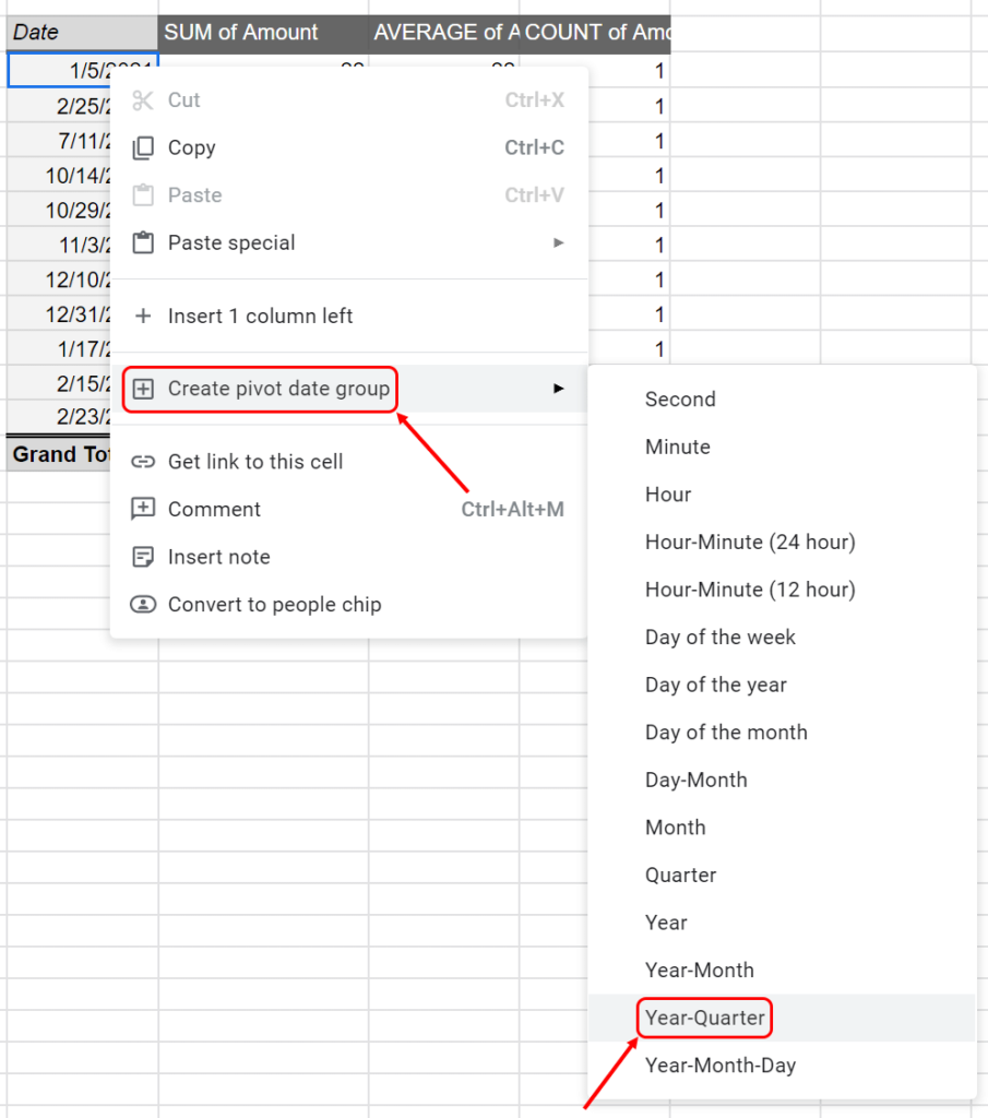
Choose the option of Year-Quarter. Choosing this will do most of the work for you that we did manually using the first method. Notice that we did not select the option of Quarter. Selecting Quarter would result in a maximum of four groups, with no separation by year. Following is the finished product using Year-Quarter .

We have a pivot table returning the same numbers as our finished formulas in example one. Notice, however, that this pivot table excludes the 2021Q2 results instead of showing zeros and an error.
Extending the Pivot Table
Now that you are using a pivot table, you can quickly introduce another grouping level. For example, you may want to see the sum of the amounts by quarter, then by Region.

This additional level of analysis only takes a minute and would be far more complicated if you used the techniques in the first example. We won’t dive too deep into using pivot tables in this tutorial, but you can learn more here.
Method 3 – Using The QUERY Function
The QUERY function is a mix of the first two methods. It is like the first method because it uses a function instead of a tool like a pivot table. Using a function means that we will not be using the menus. However, this method is like the 2nd method because it knows the meaning of a quarter, so we will not have to create a table defining quarter start and end dates.
We will be using the same source table of data as the first two methods. We have repeated it below to reduce the need to scroll through this post.
The QUERY function is quite powerful but also has a steep learning curve. However, once you understand how it works, it can be handy to create custom reports without using a pivot table. The code for the QUERY is below. Its output is in the template and the image below the code.
=QUERY(A1:D12,"select quarter(A), year(A), sum(D), avg(D), count(D) group by quarter(A), year(A) order by year(A), quarter(A)",1)

As you can see, QUERY produces a clean, easy-to-read output. You can also customize the labels for each column if you would like.
Conclusion
Now that you know three different methods to summarize spreadsheet data by quarter, you can pick which one works best for you.