Summarize Unique Values In Google Sheets

This post explains three techniques to summarize unique values in Google Sheets. Each method will list the unique values, then show a count and a sum. The three techniques increase in complexity but also in flexibility. Pick one that makes the most sense for your spreadsheet.

We will summarize the data shown below. As you can see, some items are repeated, making a total of three types of Items.

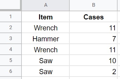
All of the techniques will use the data in this linked spreadsheet.

Video Tutorial

Using UNIQUE, SUMIF, and COUNTIF

In the first technique, we summarize unique values in the data using the UNIQUE, SUMIF, and COUNTIF functions. First, let’s create an array of the unduplicated items using the UNIQUE function.

The formula in cell A11 of =UNIQUE(A2:A6) creates an array of unique values. Wrench and Saw are duplicated in the source data but are each listed once in the output. Now that we have a list of each item let’s work on summing the number of Cases for each item. We will write the SUMIF function first.

The formula in cell B11 is =SUMIF(A$2:A$6,A11,B$2:B$6).

It uses the values in A2:A6 as the criteria range to decide if it should sum the values in B2:B6. Notice that every row number in the formula has a $ before it. Fixing the row numbers like this lets a spreadsheet user copy a formula without the row numbers shifting. Read more about how fixed cell references work in this post.

Notice we did not fix the reference to A11. Google Sheets increments the reference by one each time it is copied to the next row. Accordingly, the formula in cell B12 should reference cell A12.

Now let’s create formulas to count the values using the COUNTIF function.

The formula in cell C11 is =COUNTIF(A$2:A$6,A11).

The main difference between SUMIF and COUNTIF is that COUNTIF does not need a criteria range. We have successfully created a summary of the beginning data. This technique is familiar and easy to construct. However, if the source data changes, this method will not automatically expand to show more values. Let’s look at the second method, which is more adaptable.

Using a Pivot Table

Now let’s look at a more flexible alternative called Pivot Tables. These are dynamic tables that summarize unique values in the source data.  If you are unfamiliar with them, you can watch this video for an introduction. Pivot tables can quickly sum and count the source data above. Let’s do that now.

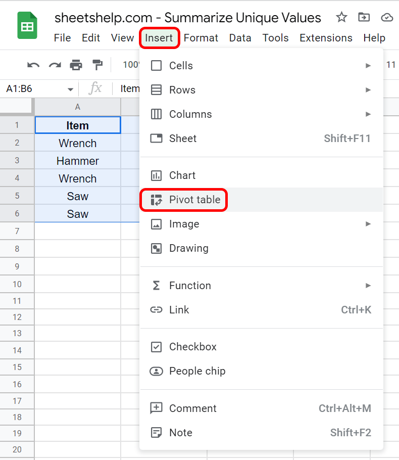
First, highlight the source data, including the headers. Then go to Insert and choose Pivot table.

Next, the Create pivot table window pops up.

The Data range value is pre-filled because we already selected the range. Use the OmniPivot add-on if you have more than one data range. Next, you can choose a location for your pivot table. I choose A8 on the same sheet because it will be easier to see in the illustrations. If the size of your raw data is likely to change, you should place your pivot table to the right of your data or on a new sheet.

Click Create, and you will see a blank pivot table and a Pivot table editor menu.

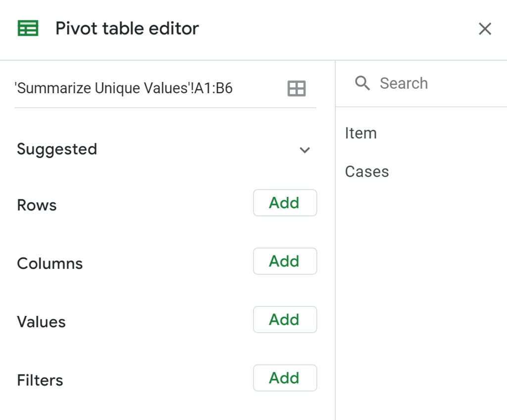
Now we can use the Pivot table editor menu to add the Item column as the Rows and Cases as the Values.

Add Cases twice to the Values field, once as a SUM and once as a COUNT. Now we have an output similar to the functions in the previous example. However, it is easier to change the functions and the source data as you won’t need to update multiple COUNTIF and SUMIF formulas as you would in the first example.

ℹ️ The pivot table is the only one of these techniques that is case-insensitive. This means that saw, with a capital letter, would be combined with Saw.

Now let’s look at the last example, which is the most powerful but also the hardest to learn.

Using the QUERY Function

The QUERY function allows us to use a function instead of the menus. However, unlike the first example, we only need one function to create the summary. A function allows us to see everything from the Formula box instead of drop-downs in the Pivot table editor menu.

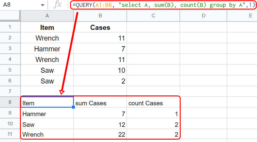
The query syntax is based on SQL and is therefore written differently than traditional functions. The As and Bs refer to the columns in the range of A1:B6. The select clause lists the output columns. A is listed as is, then B is shown as a sum and a count. Then, you tell QUERY how to group the output, and we want it by Item so we use group by A. We put it together with the following formula:

=QUERY(A1:B6, "select A, sum(B), count(B) group by A",1)

Here’s a look at it in our spreadsheet.

Conclusion – Summarize Unique Values

Now you have learned three methods to summarize unique data in your spreadsheet. Use the one that makes the most sense for you.

Related Tutorials