
The WORKDAY.INTL function calculates a future or past date based on a specified number of working days. Unlike the standard WORKDAY function, it allows you to define custom weekends (e.g., Friday-Saturday or only Sunday) and exclude a list of holidays.
If your days, months, and years are in separate cells, use the DATE function to combine them. This function is different from the WORKDAY function as you can specify other weekends.

Syntax
=WORKDAY.INTL(start_date,days,[weekend],[holidays])
start_date– The date from which to start counting.days– The number of working days to add (positive) or subtract (negative).[weekend]– (Optional) Indicates which days are weekends.- Number method: (e.g.,
1= Sat/Sun). See the Cheatsheet below. - String method: (e.g.,
"0000011"). See Example 3.
- Number method: (e.g.,
[holidays]– (Optional) A range of dates to exclude from the count.
Weekend Codes (Cheatsheet)
Use these numbers in the [weekend] argument to specify which days are off.
| Code | Weekend Days | Code | Weekend Days |
|---|---|---|---|
1 |
Saturday, Sunday (Default) | 11 |
Sunday only |
2 |
Sunday, Monday | 12 |
Monday only |
3 |
Monday, Tuesday | 13 |
Tuesday only |
4 |
Tuesday, Wednesday | 14 |
Wednesday only |
5 |
Wednesday, Thursday | 15 |
Thursday only |
6 |
Thursday, Friday | 16 |
Friday only |
7 |
Friday, Saturday | 17 |
Saturday only |
Video Tutorial

Related Functions
WEEKDAY – Returns the week number for a given date.
DAYS – Find the number of days between two dates.
NETWORKDAYS.INTL – Calculate the number of working days between two days and excludes specified days as weekends.
NETWORKDAYS – Calculate the number of working days between two days and exclude weekends.
WORKDAY – Like this function but with only Saturday and Sunday as the weekends.
Errors
#NUM – The inputs are numbers but are not valid dates. If you used the 35th day of November, “11/35/2018”, this error could happen.
#VALUE! – The inputs don’t convert to a number such as “The other day” or “Yester-yester-day.”
Examples
Example 1: 6-Day Work Week (Sunday Only Weekend)
In this scenario, a team works Monday through Saturday, with only Sunday off. We use weekend code 11.
| A | B | |
|---|---|---|
| 1 | Start Date | 1/1/2024 (Monday) |
| 2 | Days to Add | 10 |
| 3 | Result | 1/12/2024 |
| 4 | Formula | =WORKDAY.INTL(B1, B2, 11) |
Example 2: Excluding Holidays
To accurately calculate a project deadline, you must exclude holidays. In this example, we calculate 10 working days from Jan 1st, but we exclude “New Year’s Day” (Jan 1) and “MLK Day” (Jan 15).
Note: If a holiday falls on a weekend, it is not double-counted.
| A | B | C | |
|---|---|---|---|
| 1 | Start Date | 1/1/2024 | |
| 2 | Days Required | 10 | |
| 3 | Formula | =WORKDAY.INTL(B1, B2, 1, C7:C8) |
|
| 4 | Result | 1/16/2024 | |
| 5 | |||
| 6 | Holidays List | Date | Holiday Name |
| 7 | 1/1/2024 | New Year’s Day | |
| 8 | 1/15/2024 | MLK Day |
Managing Holidays (The Easy Way)
💡 Stop Typing Holidays Manually
Maintaining a list of holidays in your spreadsheet is tedious and prone to errors. Instead, import a public “Holidays” calendar directly into Sheets.
1. Subscribe to the “Holidays in United States” (or your region) calendar in Google Calendar.
2. Use the Calendar Importer Add-on to sync that calendar to your sheet.
3. Reference that imported column in yourWORKDAY.INTLformula.This ensures your project timelines are always accurate without manual updates.
Example 3: The String Method (Advanced)
If the standard numeric codes don’t fit your schedule (e.g., you work a 4-day week with Friday, Saturday, and Sunday off), you can use a binary string.
The string is 7 characters long, starting with Monday. 0 represents a workday, and 1 represents a non-working day.
Scenario: 4-Day Work Week (Fri, Sat, Sun off).
- String:
"0000111"(Mon-Thu work, Fri-Sun off)
| A | B | |
|---|---|---|
| 1 | Start Date | 1/1/2024 |
| 2 | Duration | 10 |
| 3 | Formula | =WORKDAY.INTL(B1, B2, "0000111") |
| 4 | Result | 1/18/2024 |
Example 4: Using a Named Range for the Holidays
At this point, the range for the holidays is B4:B13. But, if you wanted to reference the list from another sheet, you would need Sheet1!B4:B13 which is longer and harder to remember. Let’s make this syntax a bit cleaner with a named range. Highlight B4:B13 and type Holidays into the Name box and press Enter.

Now we can use an easier formula swapping out the B4:B13 with the named range.
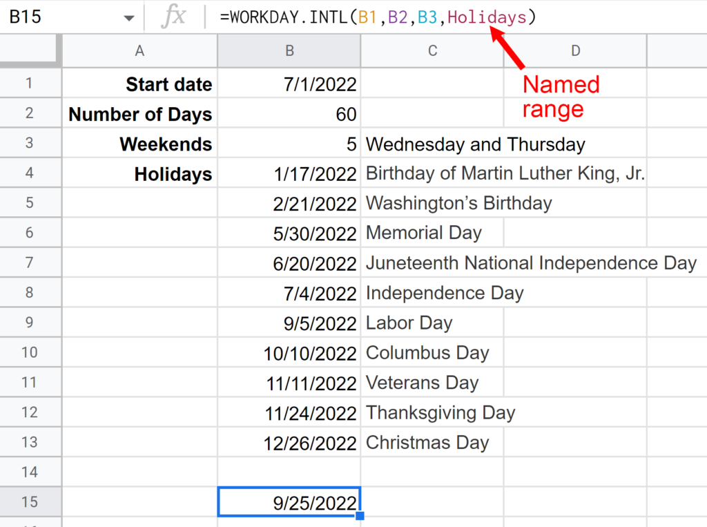
The formula of =WORKDAY.INTL(B1,B2,B3,Holidays) is the completed formula to calculate the workday sixty days away from the start date.
Live WORKDAY.INTL Examples in Sheets
Go to this spreadsheet for examples of the WORKDAY.INTL function shown above that you can study and use anywhere you would like.
Notes
Consider using the IMPORTXML function to obtain a list of your local holidays online.